1.导入CIFAR-10数据集
CIFAR-10是由 Hinton 的学生 Alex Krizhevsky 和 Ilya Sutskever 整理的一个用于识别普适物体的小型数据集。一共包含 10 个类别的 RGB 彩色图片:飞机( a叩lane )、汽车( automobile )、鸟类( bird )、猫( cat )、鹿( deer )、狗( dog )、蛙类( frog )、马( horse )、船( ship )和卡车( truck )。图片的尺寸为 32×32,3个通道 ,数据集中一共有 50000 张训练圄片和 10000 张测试图片。 CIFAR-10数据集有3个版本,这里使用python版本。
1.1 导入需要的库
|
|
import os import math import numpy as np import pickle as p import tensorflow as tf import matplotlib.pyplot as plt %matplotlib inline |
1.2 定义批量导入数据的函数
1 2 3 4 5 6 7 8 9 10 11 12 13 14 15 16 17 18 19 20 |
def load_CIFAR_batch(filename): """ load single batch of cifar """ with open(filename, 'rb')as f: # 一个样本由标签和图像数据组成 # (3072=32x32x3) # ... # data_dict = p.load(f, encoding='bytes') images= data_dict[b'data'] labels = data_dict[b'labels'] # 把原始数据结构调整为: BCWH images = images.reshape(10000, 3, 32, 32) # tensorflow处理图像数据的结构:BWHC # 把通道数据C移动到最后一个维度 images = images.transpose (0,2,3,1) labels = np.array(labels) return images, labels |
1.3 定义加载数据函数
1 2 3 4 5 6 7 8 9 10 11 12 13 14 15 16 17 18 19 20 21 |
def load_CIFAR_data(data_dir): """load CIFAR data""" images_train=[] labels_train=[] for i in range(5): f=os.path.join(data_dir,'data_batch_%d' % (i+1)) print('loading ',f) # 调用 load_CIFAR_batch( )获得批量的图像及其对应的标签 image_batch,label_batch=load_CIFAR_batch(f) images_train.append(image_batch) labels_train.append(label_batch) Xtrain=np.concatenate(images_train) Ytrain=np.concatenate(labels_train) del image_batch ,label_batch Xtest,Ytest=load_CIFAR_batch(os.path.join(data_dir,'test_batch')) print('finished loadding CIFAR-10 data') # 返回训练集的图像和标签,测试集的图像和标签 return (Xtrain,Ytrain),(Xtest,Ytest) |
1.4 加载数据
|
|
data_dir = r'data\cifar-10-batches-py' (x_train,y_train),(x_test,y_test) = load_CIFAR_data(data_dir) |
运行结果
loading data\cifar-10-batches-py\data_batch_1
loading data\cifar-10-batches-py\data_batch_2
loading data\cifar-10-batches-py\data_batch_3
loading data\cifar-10-batches-py\data_batch_4
loading data\cifar-10-batches-py\data_batch_5
finished loadding CIFAR-10 data
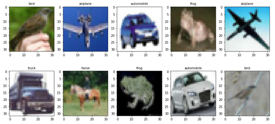
1.5 可视化加载数据
1 2 3 4 5 6 7 8 9 10 11 12 13 14 15 16 17 18 19 |
label_dict = {0:"airplane", 1:" automobile", 2:"bird", 3:"cat", 4:"deer", 5:"dog", 6:"frog", 7:"horse", 8:"ship", 9:"truck"} def plot_images_labels(images, labels, num): total = len(images) fig = plt.gcf() fig.set_size_inches(15, math.ceil(num / 10) * 7) for i in range(0, num): choose_n = np.random.randint(0, total) ax = plt.subplot(math.ceil(num / 5), 5, 1 + i) ax.imshow(images[choose_n], cmap='binary') title = label_dict[labels[choose_n]] ax.set_title(title, fontsize=10) plt.show() plot_images_labels(x_train, y_train, 10) |
运行结果
2 .数据预处理并设置超参数
|
|
x_train = x_train.astype('float32') / 255.0 x_test = x_test.astype('float32') / 255.0 train_num = len(x_train) num_classes = 10 learning_rate = 0.0002 batch_size = 64 training_steps = 20000 display_step = 1000 conv1_filters = 32 conv2_filters = 64 fc1_units = 256 |
3.使用tf.data构建数据管道
|
|
AUTOTUNE = tf.data.experimental.AUTOTUNE train_data = tf.data.Dataset.from_tensor_slices((x_train, y_train)) train_data = train_data.shuffle(5000).repeat(training_steps).batch(batch_size).prefetch(buffer_size=AUTOTUNE) |
4.定义卷积层及池化层
|
|
def conv2d(x, W, b, strides=1): #tf.nn.conv2d(input, filter, strides, padding, use_cudnn_on_gpu=None, name=None) x = tf.nn.conv2d(x, W, strides=[1, strides, strides, 1], padding='SAME') x = tf.nn.bias_add(x, b) return tf.nn.relu(x) def maxpool2d(x, k=2): #tf.nn.max_pool(value, ksize, strides, padding, name=None) return tf.nn.max_pool(x, ksize=[1, k, k, 1], strides=[1, k, k, 1], padding='SAME') |
5.构建模型
1 2 3 4 5 6 7 8 9 10 11 12 13 14 15 16 17 18 19 20 21 22 23 24 25 26 27 28 29 30 31 32 33 34 35 36 37 38 39 40 41 42 43 44 |
class CNNModel(tf.Module): def __init__(self,name = None): super(CNNModel, self).__init__(name=name) self.w1 = tf.Variable(random_normal([3, 3, 3, conv1_filters]))#[k_width, k_height, input_chn, output_chn] self.b1 = tf.Variable(tf.zeros([conv1_filters])) #输入通道:32,输出通道:64,卷积后图像尺寸不变,依然是16x16 self.w2 = tf.Variable(random_normal([3, 3, conv1_filters, conv2_filters])) self.b2 = tf.Variable(tf.zeros([conv2_filters])) #将池第2个池化层的64个8x8的图像转换为一维的向量,长度是 64*8*8=4096 self.w3 = tf.Variable(random_normal([4096, fc1_units])) self.b3 = tf.Variable(tf.zeros([fc1_units])) self.wout = tf.Variable(random_normal([fc1_units, num_classes])) self.bout = tf.Variable(tf.zeros([num_classes])) # 正向传播 def __call__(self,x): conv1 = conv2d(x, self.w1, self.b1) pool1 = maxpool2d(conv1, k=2) #将32x32图像缩小为16x16,池化不改变通道数量,因此依然是32个 conv2 = conv2d(pool1, self.w2, self.b2) pool2 = maxpool2d(conv2, k=2) flat = tf.reshape(pool2, [-1, self.w3.get_shape().as_list()[0]]) fc1 = tf.add(tf.matmul(flat, self.w3), self.b3) fc1 = tf.nn.relu(fc1) out = tf.add(tf.matmul(fc1, self.wout), self.bout) return tf.nn.softmax(out) # 损失函数(二元交叉熵) #@tf.function(input_signature=[tf.TensorSpec(shape = [None,1], dtype = tf.float32),tf.TensorSpec(shape = [None,1], dtype = tf.float32)]) def cross_entropy(self,y_pred, y_true): y_pred = tf.clip_by_value(y_pred, 1e-9, 1.) loss_ = tf.keras.losses.sparse_categorical_crossentropy(y_true=y_true, y_pred=y_pred) return tf.reduce_mean(loss_) # 评估指标(准确率) def accuracy(self,y_pred, y_true): correct_prediction = tf.equal(tf.argmax(y_pred, 1), tf.reshape(tf.cast(y_true, tf.int64), [-1])) return tf.reduce_mean(tf.cast(correct_prediction, tf.float32)) model = CNNModel() model.optimizer = tf.optimizers.Adam(learning_rate) |
6.定义训练模型函数
自定义训练过程:
(1)打开一个遍历各epoch的for循环
(2)对于每个epoch,打开一个分批遍历数据集的 for 循环
(3)对于每个批次,打开一个 GradientTape() 作用域
(4)在此作用域内,调用模型(前向传递)并计算损失
(5)在作用域之外,检索模型权重相对于损失的梯度
(6)根据梯度使用优化器来更新模型的权重
(7)评估模型指标
1 2 3 4 5 6 7 8 9 10 11 12 13 14 15 16 17 18 19 20 21 22 23 24 25 26 27 28 29 30 |
def train_step(model, features, labels): # 正向传播求损失 with tf.GradientTape() as tape: predictions = model(features) loss = model.cross_entropy(predictions,labels) # 反向传播求梯度 grads = tape.gradient(loss, model.trainable_variables) # 执行梯度下降 model.optimizer.apply_gradients(zip(grads, model.trainable_variables)) # 计算评估指标 metric = model.accuracy(predictions,labels) return loss, metric train_loss_list1 = [] train_acc_list1 = [] def train_model(model,train_data,training_steps,display_step): #for epoch in tf.range(1,epochs+1): for step, (batch_x, batch_y) in enumerate(train_data.take(training_steps), 1): starttime=time.time() loss,metric = train_step(model,batch_x,batch_y) if step % display_step == 0: #printbar() train_loss_list1.append(loss) train_acc_list1.append(metric) tf.print("step ={},loss = {:.4f},accuracy ={:.4f} ,times={:.4f}".format(step,loss,metric,(time.time() - starttime))) |
train_model(model,train_data,training_steps,display_step)
运行结果
step =1000,loss = 1.2807,accuracy =0.5781 ,times=0.0080
step =2000,loss = 1.1832,accuracy =0.6562 ,times=0.0080
step =3000,loss = 0.9727,accuracy =0.6562 ,times=0.0080
step =4000,loss = 1.0398,accuracy =0.6406 ,times=0.0050
step =5000,loss = 0.8615,accuracy =0.6406 ,times=0.0156
step =6000,loss = 0.7207,accuracy =0.7188 ,times=0.0000
step =7000,loss = 1.0945,accuracy =0.5938 ,times=0.0090
step =8000,loss = 0.7337,accuracy =0.7656 ,times=0.0080
step =9000,loss = 0.5792,accuracy =0.7812 ,times=0.0080
step =10000,loss = 0.7154,accuracy =0.7500 ,times=0.0080
step =11000,loss = 0.6398,accuracy =0.8125 ,times=0.0156
step =12000,loss = 0.6413,accuracy =0.7500 ,times=0.0080
step =13000,loss = 0.5555,accuracy =0.7812 ,times=0.0156
step =14000,loss = 0.6729,accuracy =0.8281 ,times=0.0156
step =15000,loss = 0.5163,accuracy =0.7500 ,times=0.0156
step =16000,loss = 0.5521,accuracy =0.7969 ,times=0.0000
step =17000,loss = 0.4475,accuracy =0.8594 ,times=0.0156
step =18000,loss = 0.3158,accuracy =0.8594 ,times=0.0080
step =19000,loss = 0.3829,accuracy =0.9062 ,times=0.0090
step =20000,loss = 0.2731,accuracy =0.9062 ,times=0.0080
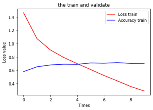
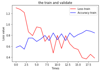
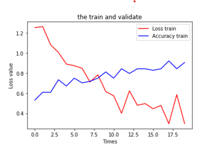
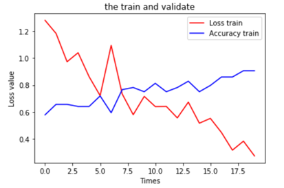
7.可视化运行结果
|
|
plt.title('the train and validate') plt.xlabel('Times') plt.ylabel('Loss value') plt.plot(train_loss_list, color=(1, 0, 0), label='Loss train') plt.plot(train_acc_list, color=(0, 0, 1), label='Accuracy train') plt.legend(loc='best') plt.show() |
8.测试型
|
|
test_total_batch = int(len(x_test) / batch_size) test_acc_sum = 0.0 for i in range(test_total_batch): test_image_batch = x_test[i*batch_size:(i+1)*batch_size] test_label_batch = y_test[i*batch_size:(i+1)*batch_size] pred = conv_net(test_image_batch) test_batch_acc = accuracy(pred,test_label_batch) test_acc_sum += test_batch_acc test_acc = float(test_acc_sum / test_total_batch) print("Test accuracy:{:.6f}".format(test_acc)) |
运行结果
Test accuracy:0.712640