第5 章 用Sklearn预测客户流失
“流失率”是描述客户离开或停止支付产品或服务费率的业务术语。这在许多企业中是一个关键的数字,因为通常情况下,获取新客户的成本比保留现有成本(在某些情况下,贵5到20倍)。
因此,了解保持客户参与度是非常宝贵的,因为它是开发保留策略和推出旨在阻止客户流失的重要基础。因此,公司对开发更好的流失检测技术愈来愈有兴趣,导致许多人寻求数据挖掘和机器学习以获得新的和创造性的方法。
5.1 导入数据集
这里我们以一个长期的电信客户数据作为数据集,您可以点击这里下载数据集。
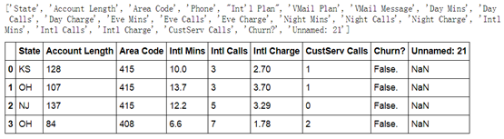
数据很简单。 每行代表一个预订的电话用户。 每列包含客户属性,例如电话号码,在一天中不同时间使用的通话分钟,服务产生的费用,生命周期帐户持续时间等。
使用pandas方便直接读取.csv里数据
import numpy as np
import matplotlib.pyplot as plt
import json
from sklearn.cross_validation import KFold
from sklearn.preprocessing import StandardScaler
from sklearn.cross_validation import train_test_split
from sklearn.svm import SVC
from sklearn.ensemble import RandomForestClassifier as RF
%matplotlib inline
churn_df = pd.read_csv('./data/customer_loss/churn.csv')
col_names = churn_df.columns.tolist()
print(col_names)
to_show = col_names[:3] + col_names[-6:]
churn_df[to_show].head(4)
显示结果如下:
5.2 预处理数据集
删除不相关的列,并将字符串转换为布尔值(因为模型不处理“yes”和“no”非常好)。 其余的数字列保持不变。
将预测结果分离转化为0,1形式,把False转换为,把True转换为1。
y = np.where(churn_result == 'True.',1,0)
y[:20]
array([0, 0, 0, 0, 0, 0, 0, 0, 0, 0, 1, 0, 0, 0, 0, 1, 0, 0, 0, 0])
删除一些不必要的特征或字段,这里是从业务角度进行取舍。
churn_feat_space = churn_df.drop(to_drop,axis=1)
将属性值yes,no等转化为boolean values,即False或True。numpy将把这些值转换为1或0.
churn_feat_space[yes_no_cols] = churn_feat_space[yes_no_cols] == 'yes'
获取新的属性和属性值。
X = churn_feat_space.as_matrix().astype(np.float)
对规模级别差距较大的数据,需要进行规范化处理。 例如:篮球队每场比赛得分的分数自然比他们的胜率要大几个数量级。 但这并不意味着后者的重要性低100倍,故需要进行标准化处理。
公式为:(X-mean)/std 计算时对每个属性/每列分别进行。
将数据按期属性(按列进行)减去其均值,并处以其方差。得到的结果是,对于每个属性/每列来说所有数据都聚集在-1到1附近,方差为1。这里直接使用sklearn库中数据预处理模块:StandardScaler
scaler = StandardScaler()
X = scaler.fit_transform(X)
打印出数据数量和属性个数及分类label。
print("Unique target labels:", np.unique(y))
Feature space holds 3332 observations and 17 features
Unique target labels: [0 1]
5.3 使用交叉验证方法
模型的性能如何?我们可通过哪些方法来验证或检验一个模型的优劣?交叉验证是一种有效方法。此外,利用交叉验证尝试避免过拟合(对同一数据点进行训练和预测),同时仍然为每个观测数据集产生预测。
交叉验证(Cross Validation)的基本思想是把在某种意义下将原始数据(dataset)进行分组,一部分做为训练集(train set),另一部分做为验证集(validation set or test set),首先用训练集对分类器进行训练,再利用验证集来测试训练得到的模型(model),以此来做为评价分类器的性能指标。
另外这里顺便介绍一下使用scikit-learn库的常用算法,如下图,接下来我们将使用多种方法来构建模型,然后比较各种算法的性能。

def run_cv(X,y,clf_class,**kwargs):
# Construct a kfolds object
kf = KFold(len(y),n_folds=5,shuffle=True)
y_pred = y.copy()
# Iterate through folds
for train_index, test_index in kf:
X_train, X_test = X[train_index], X[test_index]
y_train = y[train_index]
# Initialize a classifier with key word arguments
clf = clf_class(**kwargs)
clf.fit(X_train,y_train)
y_pred[test_index] = clf.predict(X_test)
return y_pred
5.4 训练模型
比较三个相当独特的算法:支持向量机,集成方法,随机森林和k最近邻。 然后,显示各分类器预测正确率。
from sklearn.ensemble import RandomForestClassifier as RF
from sklearn.neighbors import KNeighborsClassifier as KNN
from sklearn.linear_model import LogisticRegression as LR
from sklearn.ensemble import GradientBoostingClassifier as GBC
from sklearn.metrics import average_precision_score
def accuracy(y_true,y_pred):
# NumPy interpretes True and False as 1. and 0.
return np.mean(y_true == y_pred)
print( "Logistic Regression:")
print( "%.3f" % accuracy(y, run_cv(X,y,LR)))
print( "Gradient Boosting Classifier")
print( "%.3f" % accuracy(y, run_cv(X,y,GBC)))
print( "Support vector machines:")
print( "%.3f" % accuracy(y, run_cv(X,y,SVC)))
print( "Random forest:")
print( "%.3f" % accuracy(y, run_cv(X,y,RF)))
print( "K-nearest-neighbors:")
print( "%.3f" % accuracy(y, run_cv(X,y,KNN)))
Logistic Regression:
0.862
Gradient Boosting Classifier
0.951
Support vector machines:
0.922
Random forest:
0.942
K-nearest-neighbors:
0.893
可以看出Gradient Boosting、Random forest性能较好。
5.5 精确率和召回率
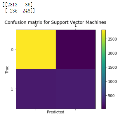
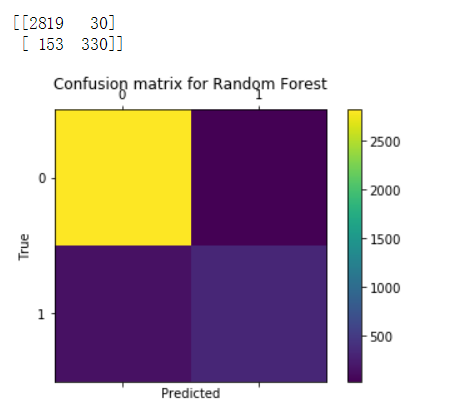
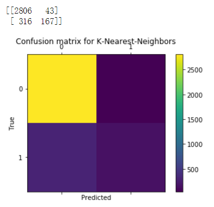
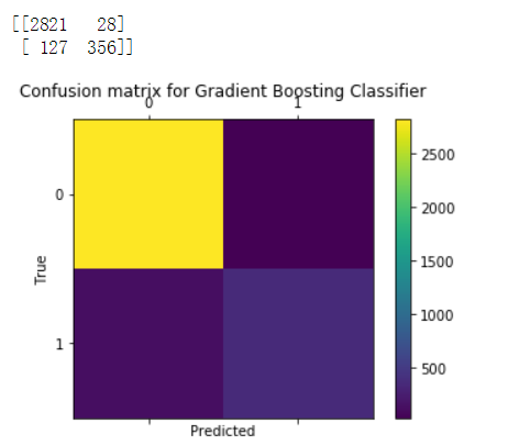
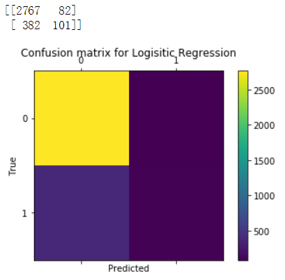
评估模型有很多方法,对分类问题,尤其是二分类问题通常采用准确率和召回率来衡量。这里我们将使用scikit-learn一个内置的函数来构造混淆矩阵。该矩阵反应模型的这些指标。混淆矩阵是一种可视化由分类器进行的预测的方式,并且仅仅是一个表格,其示出了对于特定类的预测的分布。 x轴表示每个观察的真实类别(如果客户流失或不流失),而y轴对应于模型预测的类别(如果我的分类器表示客户会流失或不流失)。这里补充一下有关混淆矩阵的有关定义,供大家参考。
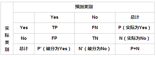
二元分类的混淆矩阵形式如下:
True Positive(真正,TP):将正类预测为正类数;
True Negative(真负,TN):将负类预测为负类数;
False Positive(假正,FP):将负类预测为正类数误报 (Type I error);
False Negative(假负,FN):将正类预测为负类数→漏报 (Type II error)

混淆矩阵的缺点:
一些positive事件发生概率极小的不平衡数据集(imbalanced data),混淆矩阵可能效果不好。比如对信用卡交易是否异常做分类的情形,很可能1万笔交易中只有1笔交易是异常的。一个将所有交易都判定为正常的分类器,准确率是99.99%。这个数字虽然很高,但是没有任何现实意义。
from sklearn.metrics import precision_score
from sklearn.metrics import recall_score
def draw_confusion_matrices(confusion_matricies,class_names):
class_names = class_names.tolist()
for cm in confusion_matrices:
classifier, cm = cm[0], cm[1]
print(cm)
fig = plt.figure()
ax = fig.add_subplot(111)
cax = ax.matshow(cm)
plt.title('Confusion matrix for %s' % classifier)
fig.colorbar(cax)
ax.set_xticklabels([''] + class_names)
ax.set_yticklabels([''] + class_names)
plt.xlabel('Predicted')
plt.ylabel('True')
plt.show()
y = np.array(y)
class_names = np.unique(y)
confusion_matrices = [
( "Support Vector Machines", confusion_matrix(y,run_cv(X,y,SVC)) ),
( "Random Forest", confusion_matrix(y,run_cv(X,y,RF)) ),
( "K-Nearest-Neighbors", confusion_matrix(y,run_cv(X,y,KNN)) ),
( "Gradient Boosting Classifier", confusion_matrix(y,run_cv(X,y,GBC)) ),
( "Logisitic Regression", confusion_matrix(y,run_cv(X,y,LR)) )
]
# Pyplot code not included to reduce clutter
# from churn_display import draw_confusion_matrices
%matplotlib inline
draw_confusion_matrices(confusion_matrices,class_names)
5.6 ROC & AUC
这里我们简单介绍一下这两个概念。
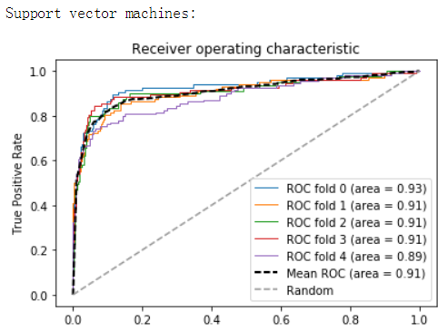
ROC曲线是根据一系列不同的二分类方式(分界值或决定阈),以真阳性率(灵敏度)为纵坐标,假阳性率(1-特异度)为横坐标绘制的曲线。传统的诊断试验评价方法有一个共同的特点,必须将试验结果分为两类,再进行统计分析。ROC曲线的评价方法与传统的评价方法不同,无须此限制,而是根据实际情况,允许有中间状态,可以把试验结果划分为多个有序分类,如正常、大致正常、可疑、大致异常和异常五个等级再进行统计分析。因此,ROC曲线评价方法适用的范围更为广泛
AUC值为ROC曲线所覆盖的区域面积,显然,AUC越大,分类器分类效果越好。
from scipy import interp
def plot_roc(X, y, clf_class, **kwargs):
kf = KFold(len(y), n_folds=5, shuffle=True)
y_prob = np.zeros((len(y),2))
mean_tpr = 0.0
mean_fpr = np.linspace(0, 1, 100)
all_tpr = []
for i, (train_index, test_index) in enumerate(kf):
X_train, X_test = X[train_index], X[test_index]
y_train = y[train_index]
clf = clf_class(**kwargs)
clf.fit(X_train,y_train)
# Predict probabilities, not classes
y_prob[test_index] = clf.predict_proba(X_test)
fpr, tpr, thresholds = roc_curve(y[test_index], y_prob[test_index, 1])
mean_tpr += interp(mean_fpr, fpr, tpr)
mean_tpr[0] = 0.0
roc_auc = auc(fpr, tpr)
plt.plot(fpr, tpr, lw=1, label='ROC fold %d (area = %0.2f)' % (i, roc_auc))
mean_tpr /= len(kf)
mean_tpr[-1] = 1.0
mean_auc = auc(mean_fpr, mean_tpr)
plt.plot(mean_fpr, mean_tpr, 'k--',label='Mean ROC (area = %0.2f)' % mean_auc, lw=2)
plt.plot([0, 1], [0, 1], '--', color=(0.6, 0.6, 0.6), label='Random')
plt.xlim([-0.05, 1.05])
plt.ylim([-0.05, 1.05])
plt.xlabel('False Positive Rate')
plt.ylabel('True Positive Rate')
plt.title('Receiver operating characteristic')
plt.legend(loc="lower right")
plt.show()
print("Support vector machines:")
print(plot_roc(X,y,SVC,probability=True))
print("Random forests:")
print(plot_roc(X,y,RF,n_estimators=18))
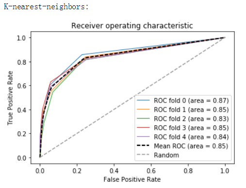
print("K-nearest-neighbors:")
print(plot_roc(X,y,KNN))
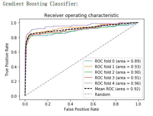
print("Gradient Boosting Classifier:")
print(plot_roc(X,y,GBC))

5.7 特征分析
我们想进一步分析,流失客户有哪些比较明显的特征。或哪些特征对客户流失影响比较大。
forest = RF()
forest_fit = forest.fit(X[train_index], y[train_index])
forest_predictions = forest_fit.predict(X[test_index])
importances = forest_fit.feature_importances_[:10]
std = np.std([tree.feature_importances_ for tree in forest.estimators_],
axis=0)
indices = np.argsort(importances)[::-1]
# Print the feature ranking
print("Feature ranking:")
for f in range(10):
#print("%d. %s (%f)" % (f + 1, features[f], importances[indices[f]]))
print("%d. %s (%f)" % (f + 1, features[f], importances[f]))
# Plot the feature importances of the forest
#import pylab as pl
plt.figure()
plt.title("Feature importances")
plt.bar(range(10), importances[indices], yerr=std[indices], color="r", align="center")
plt.xticks(range(10), indices)
plt.xlim([-1, 10])
plt.show()
Feature ranking:
1. Account Length (0.026546)
2. Int'l Plan (0.054757)
3. VMail Plan (0.020334)
4. VMail Message (0.041116)
5. Day Mins (0.164627)
6. Day Calls (0.026826)
7. Day Charge (0.120162)
8. Eve Mins (0.086248)
9. Eve Calls (0.022896)
10. Eve Charge (0.046945)
def run_prob_cv(X, y, clf_class, roc=False, **kwargs):
kf = KFold(len(y), n_folds=5, shuffle=True)
y_prob = np.zeros((len(y),2))
for train_index, test_index in kf:
X_train, X_test = X[train_index], X[test_index]
y_train = y[train_index]
clf = clf_class(**kwargs)
clf.fit(X_train,y_train)
# Predict probabilities, not classes
y_prob[test_index] = clf.predict_proba(X_test)
return y_prob
warnings.filterwarnings('ignore')
# Use 10 estimators so predictions are all multiples of 0.1
pred_prob = run_prob_cv(X, y, RF, n_estimators=10)
pred_churn = pred_prob[:,1]
is_churn = y == 1
# Number of times a predicted probability is assigned to an observation
counts = pd.value_counts(pred_churn)
counts[:]
0.0 1782
0.1 666
0.2 276
0.3 123
0.9 89
0.4 85
0.7 73
0.8 65
1.0 63
0.6 61
0.5 49
dtype: int64
true_prob = defaultdict(float)
# calculate true probabilities
for prob in counts.index:
true_prob[prob] = np.mean(is_churn[pred_churn == prob])
true_prob = pd.Series(true_prob)
# pandas-fu
counts = pd.concat([counts,true_prob], axis=1).reset_index()
counts.columns = ['pred_prob', 'count', 'true_prob']
counts

我们可以看到,随机森林预测89个人将有0.9的可能性的流失,而在现实中,该群体具有大约0.98的流失率。
参考:
http://www.sohu.com/a/149724745_99906660
http://nbviewer.jupyter.org/github/donnemartin/data-science-ipython-notebooks/blob/master/analyses/churn.ipynb
Pingback引用通告: Python与人工智能 – 飞谷云人工智能