文章目录
第14章 由浅入深--轻松学会--用Python实现神经网络
我们知道现在神经网络很火,功能很强大、运用范围也很广泛,所以很多人都想在神经网络这方面有所突破和进展。但有不少读者,苦于基础不够,进展一致不尽人意。我们这一章或许能提高您的学习效率,使您能更快了解神经网络的架构和原理,并逐渐自己写神经网络算法。
本章我们将由浅入深介绍用Python实现神经网络,首先介绍感知器的实现方法,然后,介绍一种激活函数为恒等式的自适应神经网络算法,最后,介绍含隐含层的多层神经网络算法。学好这些算法将为学习深度学习打下扎实基础。
14.1 使用Python实现感知器学习算法
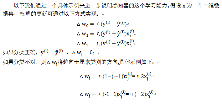
这里我们使用弗兰克•罗森布拉特(Frank Rossenblatt)提出的一个感知器,这类感知器有一个自学习算法,该算法可以自动通过优化得到权重系数,此权重系统与输入值的乘积决定神经元是否被激活。其权重更新无需损失函数,当然更无需求导,所以非常简单。
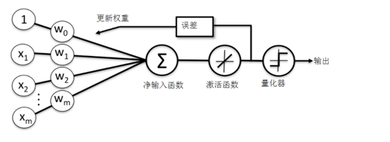
14.1.1感知器简单结构

这里净输入函数为输入样本x与权重值w的相乘后的累加,假设:

分段函数ϕ(z)用图形可表示为:

14.1.2 感知器算法步骤

14.1.3 用Python实现感知器算法
这里使用的数据为鸢尾花数据集,定义感知器类(perceptron),在这个类中定义一个从数据中进行学习的fit方法,使用predict方法进行预测。对非初始化定义的变量,为区别起见我们将假设一个下划线,如self.w_。
1)定义感知器类
定义一个感知器类,在这个类中,先定义两个参数:学习速率eta,迭代步数n_iter;然后定义了两个属性:每次训练样本时记录权重的1维向量w_,用于记录每次迭代时发生错误的样本数errors_;在这个基础上定义了用来训练数据集的函数fit,计算净输入函数net_input,用于预测的函数predict。
class Perceptron(object):
"""参数
eta : float
学习速率 (between 0.0 and 1.0)
n_iter : int
迭代步数.
属性:
w_ : 1d-array,训练后记录权重.
errors_ : list,记录每次迭代的错误数.
"""
def __init__(self, eta=0.01, n_iter=10):
self.eta = eta
self.n_iter = n_iter
def fit(self, X, y):
"""Fit training data.
Parameters
----------
X : {array-like}, shape = [n_samples, n_features]
Training vectors, where n_samples is the number of samples and
n_features is the number of features.
y : array-like, shape = [n_samples]
Target values.
Returns
-------
self : object
"""
self.w_ = np.zeros(1 + X.shape[1])
self.errors_ = []
for _ in range(self.n_iter):
errors = 0
for xi, target in zip(X, y):
update = self.eta * (target - self.predict(xi))
self.w_[1:] += update * xi
self.w_[0] += update
errors += int(update != 0.0)
self.errors_.append(errors)
return self
def net_input(self, X):
"""计算输入"""
return np.dot(X, self.w_[1:]) + self.w_[0]
def predict(self, X):
"""Return class label after unit step"""
return np.where(self.net_input(X) >= 0.0, 1, -1)
2)导入鸢尾花数据集
该数据集前4列为特征,最后1列为类别。
df = pd.read_csv('https://archive.ics.uci.edu/ml/'
'machine-learning-databases/iris/iris.data', header=None)
df.tail()

3)可视化数据集
为便于可视化及使用二分类(实际也可以使用多分类),这里我们只取前100个类标,其中前50个为山鸢尾类标,后50个为变色鸢尾类标,类标赋给向量y。提取这100个样本中第1、3个特征,并赋值给矩阵X。
import matplotlib.pyplot as plt
import numpy as np
#显示中文
import matplotlib.font_manager as fm
myfont = fm.FontProperties(fname='/home/hadoop/anaconda3/lib/python3.6/site-packages/matplotlib/mpl-data/fonts/ttf/simhei.ttf')
# select setosa and versicolor
y = df.iloc[0:100, 4].values
y = np.where(y == 'Iris-setosa', -1, 1)
# extract sepal length and petal length
X = df.iloc[0:100, [0, 2]].values
# plot data
plt.scatter(X[:50, 0], X[:50, 1],
color='red', marker='o', label='setosa')
plt.scatter(X[50:100, 0], X[50:100, 1],
color='blue', marker='x', label='versicolor')
plt.xlabel('花瓣长度[cm]',fontproperties=myfont)
plt.ylabel('萼片长度[cm]',fontproperties=myfont)
plt.legend(loc='upper left')
plt.tight_layout()
plt.show()

4)利用鸢尾花数据集训练感知器,并同时绘制每次迭代的错误分类数量。
ppn.fit(X, y)
plt.plot(range(1, len(ppn.errors_) + 1), ppn.errors_, marker='o')
plt.xlabel('迭代次数',fontproperties=myfont)
plt.ylabel('错误分类样本数',fontproperties=myfont)
plt.tight_layout()
plt.show()
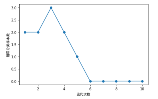
如上图所示,我们的分类器在第6次迭代后,错误数就为0,说明已收敛了。
14.2 使用Python实现自适应线性神经网络
第1节我们介绍使用Python实现一个单层的感知器神经网络,其激活函数为一个分段函数,这里我们介绍的自适应(Adaline)线性神经网络,其激活函数为一个恒等式。这个可以认为是对前一章神经网络的改进。其权重更新采用了一个连续的线性激活函数(一个恒等函数)来完成,而不是基于分段函数。Adaline算法中作用于净输入的激活函数ϕ(z)是个简单的线性恒等式,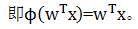 。
。
14.2.1 自适应线性神经网络结构
线性激活函数在更新权重的同时,我们使用量化器对类标进行预测,量化器与上节的单位分段函数类似,自适应线性神经网络的结构如下图所示:
14.2.2 通过梯度下降法最小化损失函数
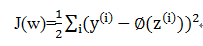
在机器学习中一个最核心的内容就是如何定义一个损失函数及优化损失函数,在自适应算法中,我们可以把模型输出值与实际类标之间的误差平方和(SSE),具体公式如下:
与单位阶跃函数相比,这种连续型激活函数有几个有点:
1)损失函数可导
2)损失函数是一个凸函数,可以通过梯度下降法更新权重,并获取全局最小值。
当然也有一些缺点,线性激活函数无法对非线性数据集进行划分,这点后续我们会介绍。
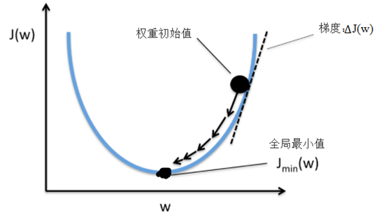
这里采用梯度下降法(如下图)来最小化损失函数J(w), 首先来看看梯度下降的一个直观的解释。比如我们在一座大山上的某处位置,由于我们不知道怎么下山,于是决定走一步算一步,先确定一个初始位置,然后求解当前位置的梯度,沿着梯度的负方向,也就是当前最陡峭的位置向下走一步,然后继续求解当前位置梯度,向这一步所在位置沿着最陡峭最易下山的位置走一步。这样一步步的走下去,一直走到觉得我们已经到了山脚。当然这样走下去,有可能我们不能走到山脚,而是到了某一个局部的山峰低处。
从上面的解释可以看出,梯度下降不一定能够找到全局的最优解,有可能是一个局部最优解。当然,如果损失函数是凸函数,梯度下降法得到的解就一定是全局最优解。所以我们这里的选择凸函数作为我们的损失函数,这是重要考量之一。
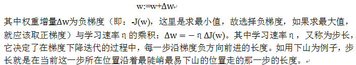
通过梯度下降,我们可以基于损失函数J(w)沿着梯度∆J(w)方向做一次权重更新:
为求损失函数的梯度,我们需要计算损失函数对于每个权重w_j的偏导:

14.2.3 使用Python实现自适应线性神经网络

import matplotlib.pyplot as plt
import numpy as np
import pandas as pd
#显示中文
import matplotlib.font_manager as fm
myfont = fm.FontProperties(fname='/home/hadoop/anaconda3/lib/python3.6/site-packages/matplotlib/mpl-data/fonts/ttf/simhei.ttf')
df = pd.read_csv('https://archive.ics.uci.edu/ml/'
'machine-learning-databases/iris/iris.data', header=None)
# select setosa and versicolor
y = df.iloc[0:100, 4].values
y = np.where(y == 'Iris-setosa', -1, 1)
# extract sepal length and petal length
X = df.iloc[0:100, [0, 2]].values
#对特征进行标准化处理
X_std = np.copy(X)
X_std[:,0] = (X[:,0] - X[:,0].mean()) / X[:,0].std()
X_std[:,1] = (X[:,1] - X[:,1].mean()) / X[:,1].std()
#fig, ax = plt.subplots(nrows=1, ncols=1, figsize=(8, 4))
ada1 = AdalineGD(n_iter=20, eta=0.01).fit(X_std, y)
plt.plot(range(1, len(ada1.cost_) + 1), np.log10(ada1.cost_), marker='o')
plt.xlabel('迭代次数',fontproperties=myfont)
plt.ylabel('log(均方根误差)',fontproperties=myfont)
plt.title('Adaline - 学习速率 0.01',fontproperties=myfont)
plt.tight_layout()
plt.show()

从以上图形可以看出,Adaline算法收敛效果不错,迭代到15次后,损失函数逐渐收敛。
【延伸思考】
1)、大家可以调整学习速率这个参数,分几种情况,如大于0.01或小于0.01的情况,然后看一下收敛情况。
2)、这里学习速率是固定不变,我们是否可以在迭代过程中动态调整这个参数?如何调整?
3)这里我们是一次训练整个数据集,如果数据集不大,还可以。如果数据量很大,这种方法就可能带来性能问题。对于大数据集对此,是否可以采用分批训练?如何实现,不妨动手尝试一下。
14.3 用Python实现多层神经网络
前面两节,我们分别介绍了感知器神经网络(Rossenblatt提出的)、自适应线性神经网络(Adaline),这两种虽然有激活函数,但只有输入层和输出层,没有隐含层,所以一般称为单层神经网络,这节我们将介绍一种含隐含层的神经网络,这样就有三层,分别为输入层、隐含层、输出层,隐含层的所有单元连接到输入层上,输出层的所有单元也全连接到隐含层中,如下图所示:如下图:
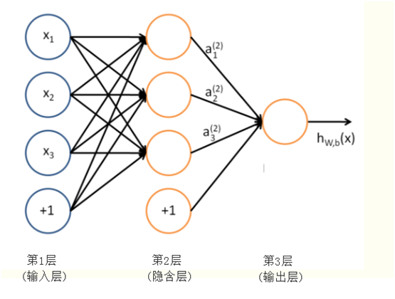
图 三层神经网络
14.3 三层神经网络介绍
下图为典型的三层神经网络的基本构成,由输入层、隐含层、输出层构成,激活函数取sigmoid函数:

的图形为S型曲线,其输出介于[0,1]之间,如下图:

sigmoid函数的导数比较有特色,下面我们简单演示一下其求导过程:

14.3.1 正向传播构造神经网络
为便于后续标识统一起见,我们使用Numpy中的向量化的代码,不使用一般的循环方法,所以基本从矩阵或向量的角度考虑各个节点的数据,具体设置如下:
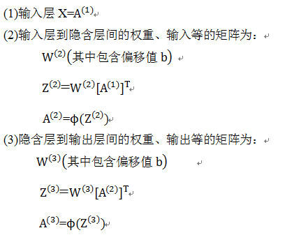
这些矩阵或向量的具体位置,可参考下图:

有了上面这些设置后,我们就可方便设计出这个神经网络的前向传导算法的步骤:

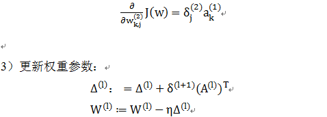
14.3.2 反向传播构造神经网络
反向传播算法(BP算法)与前向传导算法的方向正好相反,前向传导是从左到右,反向传播算法是从右到左。前向传导把激活值往后传导,反向传播则往前传播梯度,并更新权重参数。
传播的梯度将使损失函数最小化,这里的损失函数我们采用交叉熵函数:

14.3.3 用Python实现前向传导与反向传播算法
这里以MNIST为数据集,MNIST是一个手写数字0-9的数据集,它有60000个训练样本集和10000个测试样本集它是NIST数据库的一个子集。
MNIST数据库官方网址为:http://yann.lecun.com/exdb/mnist/ ,也可以在windows下直接下载,train-images-idx3-ubyte.gz、train-labels-idx1-ubyte.gz等。下载四个文件,可用
gzip *ubyte.gz -d 解压缩。解压缩后发现这些文件并不是标准的图像格式。这些图像数据都保存在二进制文件中。每个样本图像的宽高为28*28。
14.3.4 导入数据
import struct
import numpy as np
def load_mnist(path, kind='train'):
"""Load MNIST data from <code>path</code>"""
labels_path = os.path.join(path,
'%s-labels-idx1-ubyte'
% kind)
images_path = os.path.join(path,
'%s-images-idx3-ubyte'
% kind)
with open(labels_path, 'rb') as lbpath:
magic, n = struct.unpack('>II',
lbpath.read(8))
labels = np.fromfile(lbpath,
dtype=np.uint8)
with open(images_path, 'rb') as imgpath:
magic, num, rows, cols = struct.unpack(">IIII",
imgpath.read(16))
images = np.fromfile(imgpath,
dtype=np.uint8).reshape(len(labels), 784)
return images, labels
14.3.5 获取训练及测试数据
print('Rows: %d, columns: %d' % (X_train.shape[0], X_train.shape[1]))
X_test, y_test = load_mnist('./data/mnist', kind='t10k')
print('Rows: %d, columns: %d' % (X_test.shape[0], X_test.shape[1]))
import matplotlib.pyplot as plt
%matplotlib inline
fig, ax = plt.subplots(nrows=2, ncols=5, sharex=True, sharey=True,)
ax = ax.flatten()
for i in range(10):
img = X_train[y_train == i][0].reshape(28, 28)
ax[i].imshow(img, cmap='Greys', interpolation='nearest')
ax[0].set_xticks([])
ax[0].set_yticks([])
plt.tight_layout()
plt.show()
<img src="http://www.feiguyunai.com/wp-content/uploads/2017/11/8ab93c7d758f8861c54f132165ba8e93.png" alt="" />
<h3>14.3.6 定义多层神经网络</h3>
import numpy as np
from scipy.special import expit
import sys
class NeuralNetMLP(object):
""" Feedforward neural network / Multi-layer perceptron classifier.
Parameters
------------
n_output : int
Number of output units, should be equal to the
number of unique class labels.
n_features : int
Number of features (dimensions) in the target dataset.
Should be equal to the number of columns in the X array.
n_hidden : int (default: 30)
Number of hidden units.
l1 : float (default: 0.0)
Lambda value for L1-regularization.
No regularization if l1=0.0 (default)
l2 : float (default: 0.0)
Lambda value for L2-regularization.
No regularization if l2=0.0 (default)
epochs : int (default: 500)
Number of passes over the training set.
eta : float (default: 0.001)
Learning rate.
alpha : float (default: 0.0)
Momentum constant. Factor multiplied with the
gradient of the previous epoch t-1 to improve
learning speed
w(t) := w(t) - (grad(t) + alpha*grad(t-1))
decrease_const : float (default: 0.0)
Decrease constant. Shrinks the learning rate
after each epoch via eta / (1 + epoch*decrease_const)
shuffle : bool (default: True)
Shuffles training data every epoch if True to prevent circles.
minibatches : int (default: 1)
Divides training data into k minibatches for efficiency.
Normal gradient descent learning if k=1 (default).
random_state : int (default: None)
Set random state for shuffling and initializing the weights.
Attributes
-----------
cost_ : list
Sum of squared errors after each epoch.
"""
def __init__(self, n_output, n_features, n_hidden=30,
l1=0.0, l2=0.0, epochs=500, eta=0.001,
alpha=0.0, decrease_const=0.0, shuffle=True,
minibatches=1, random_state=None):
np.random.seed(random_state)
self.n_output = n_output
self.n_features = n_features
self.n_hidden = n_hidden
self.w2, self.w3 = self._initialize_weights()
self.l1 = l1
self.l2 = l2
self.epochs = epochs
self.eta = eta
self.alpha = alpha
self.decrease_const = decrease_const
self.shuffle = shuffle
self.minibatches = minibatches
def _encode_labels(self, y, k):
"""Encode labels into one-hot representation
Parameters
------------
y : array, shape = [n_samples]
Target values.
Returns
-----------
onehot : array, shape = (n_labels, n_samples)
"""
onehot = np.zeros((k, y.shape[0]))
for idx, val in enumerate(y):
onehot[val, idx] = 1.0
return onehot
def _initialize_weights(self):
"""Initialize weights with small random numbers."""
w2 = np.random.uniform(-1.0, 1.0, size=self.n_hidden*(self.n_features + 1))
w2 = w2.reshape(self.n_hidden, self.n_features + 1)
w3 = np.random.uniform(-1.0, 1.0, size=self.n_output*(self.n_hidden + 1))
w3 = w3.reshape(self.n_output, self.n_hidden + 1)
return w2, w3
def _sigmoid(self, z):
"""Compute logistic function (sigmoid)
Uses scipy.special.expit to avoid overflow
error for very small input values z.
"""
# return 1.0 / (1.0 + np.exp(-z))
return expit(z)
def _sigmoid_gradient(self, z):
"""Compute gradient of the logistic function"""
sg = self._sigmoid(z)
return sg * (1 - sg)
def _add_bias_unit(self, X, how='column'):
"""Add bias unit (column or row of 1s) to array at index 0"""
if how == 'column':
X_new = np.ones((X.shape[0], X.shape[1]+1))
X_new[:, 1:] = X
elif how == 'row':
X_new = np.ones((X.shape[0]+1, X.shape[1]))
X_new[1:, :] = X
else:
raise AttributeError('<code>how</code> must be <code>column</code> or <code>row</code>')
return X_new
def _feedforward(self, X, w2, w3):
"""Compute feedforward step
Parameters
-----------
X : array, shape = [n_samples, n_features]
Input layer with original features.
w2 : array, shape = [n_hidden_units, n_features]
Weight matrix for input layer -> hidden layer.
w3 : array, shape = [n_output_units, n_hidden_units]
Weight matrix for hidden layer -> output layer.
Returns
----------
a1 : array, shape = [n_samples, n_features+1]
Input values with bias unit.
z2 : array, shape = [n_hidden, n_samples]
Net input of hidden layer.
a2 : array, shape = [n_hidden+1, n_samples]
Activation of hidden layer.
z3 : array, shape = [n_output_units, n_samples]
Net input of output layer.
a3 : array, shape = [n_output_units, n_samples]
Activation of output layer.
"""
a1 = self._add_bias_unit(X, how='column')
z2 = w2.dot(a1.T)
a2 = self._sigmoid(z2)
a2 = self._add_bias_unit(a2, how='row')
z3 = w3.dot(a2)
a3 = self._sigmoid(z3)
return a1, z2, a2, z3, a3
def _L2_reg(self, lambda_, w2, w3):
"""Compute L2-regularization cost"""
return (lambda_/2.0) * (np.sum(w2[:, 1:] ** 2) + np.sum(w3[:, 1:] ** 2))
def _L1_reg(self, lambda_, w2, w3):
"""Compute L1-regularization cost"""
return (lambda_/2.0) * (np.abs(w2[:, 1:]).sum() + np.abs(w3[:, 1:]).sum())
def _get_cost(self, y_enc, output, w2, w3):
"""Compute cost function.
y_enc : array, shape = (n_labels, n_samples)
one-hot encoded class labels.
output : array, shape = [n_output_units, n_samples]
Activation of the output layer (feedforward)
w2 : array, shape = [n_hidden_units, n_features]
Weight matrix for input layer -> hidden layer.
w3 : array, shape = [n_output_units, n_hidden_units]
Weight matrix for hidden layer -> output layer.
Returns
---------
cost : float
Regularized cost.
"""
term1 = -y_enc * (np.log(output))
term2 = (1 - y_enc) * np.log(1 - output)
cost = np.sum(term1 - term2)
L1_term = self._L1_reg(self.l1, w2, w3)
L2_term = self._L2_reg(self.l2, w2, w3)
cost = cost + L1_term + L2_term
return cost
def _get_gradient(self, a1, a2, a3, z2, y_enc, w2, w3):
""" Compute gradient step using backpropagation.
Parameters
------------
a1 : array, shape = [n_samples, n_features+1]
Input values with bias unit.
a2 : array, shape = [n_hidden+1, n_samples]
Activation of hidden layer.
a3 : array, shape = [n_output_units, n_samples]
Activation of output layer.
z2 : array, shape = [n_hidden, n_samples]
Net input of hidden layer.
y_enc : array, shape = (n_labels, n_samples)
one-hot encoded class labels.
w2 : array, shape = [n_hidden_units, n_features]
Weight matrix for input layer -> hidden layer.
w3 : array, shape = [n_output_units, n_hidden_units]
Weight matrix for hidden layer -> output layer.
Returns
---------
grad1 : array, shape = [n_hidden_units, n_features]
Gradient of the weight matrix w2.
grad2 : array, shape = [n_output_units, n_hidden_units]
Gradient of the weight matrix w3.
"""
# backpropagation
sigma3 = a3 - y_enc
z2 = self._add_bias_unit(z2, how='row')
sigma2 = w3.T.dot(sigma3) * self._sigmoid_gradient(z2)
sigma2 = sigma2[1:, :]
grad1 = sigma2.dot(a1)
grad2 = sigma3.dot(a2.T)
# regularize
grad1[:, 1:] += (w2[:, 1:] * (self.l1 + self.l2))
grad2[:, 1:] += (w3[:, 1:] * (self.l1 + self.l2))
return grad1, grad2
def predict(self, X):
"""Predict class labels
Parameters
-----------
X : array, shape = [n_samples, n_features]
Input layer with original features.
Returns:
----------
y_pred : array, shape = [n_samples]
Predicted class labels.
"""
if len(X.shape) != 2:
raise AttributeError('X must be a [n_samples, n_features] array.\n'
'Use X[:,None] for 1-feature classification,'
'\nor X[[i]] for 1-sample classification')
a1, z2, a2, z3, a3 = self._feedforward(X, self.w2, self.w3)
y_pred = np.argmax(z3, axis=0)
return y_pred
def fit(self, X, y, print_progress=False):
""" Learn weights from training data.
Parameters
-----------
X : array, shape = [n_samples, n_features]
Input layer with original features.
y : array, shape = [n_samples]
Target class labels.
print_progress : bool (default: False)
Prints progress as the number of epochs
to stderr.
Returns:
----------
self
"""
self.cost_ = []
X_data, y_data = X.copy(), y.copy()
y_enc = self._encode_labels(y, self.n_output)
delta_w2_prev = np.zeros(self.w2.shape)
delta_w3_prev = np.zeros(self.w3.shape)
for i in range(self.epochs):
# adaptive learning rate
self.eta /= (1 + self.decrease_const*i)
if print_progress:
sys.stderr.write('\rEpoch: %d/%d' % (i+1, self.epochs))
sys.stderr.flush()
if self.shuffle:
idx = np.random.permutation(y_data.shape[0])
X_data, y_enc = X_data[idx], y_enc[:, idx]
mini = np.array_split(range(y_data.shape[0]), self.minibatches)
for idx in mini:
# feedforward
a1, z2, a2, z3, a3 = self._feedforward(X_data[idx], self.w2, self.w3)
cost = self._get_cost(y_enc=y_enc[:, idx],
output=a3,
w2=self.w2,
w3=self.w3)
self.cost_.append(cost)
# compute gradient via backpropagation
grad1, grad2 = self._get_gradient(a1=a1, a2=a2,
a3=a3, z2=z2,
y_enc=y_enc[:, idx],
w2=self.w2,
w3=self.w3)
delta_w2, delta_w3 = self.eta * grad1, self.eta * grad2
self.w2 -= (delta_w2 + (self.alpha * delta_w2_prev))
self.w3 -= (delta_w3 + (self.alpha * delta_w3_prev))
delta_w2_prev, delta_w3_prev = delta_w2, delta_w3
return self
【备注】程序具体实现时,做了一些优化,如正则化,自适应学习速率等。
14.3.7 训练模型
训练模型
n_features=X_train.shape[1],
n_hidden=50,
l2=0.1,
l1=0.0,
epochs=1000,
eta=0.001,
alpha=0.001,
decrease_const=0.00001,
minibatches=50,
shuffle=True,
random_state=1)
nn.fit(X_train, y_train, print_progress=True)
<h3>14.3.8 可视化训练结果</h3>
%matplotlib inline
import matplotlib.pyplot as plt
plt.plot(range(len(nn.cost_)), nn.cost_)
plt.ylim([0, 2000])
plt.ylabel('Cost')
plt.xlabel('Epochs * 50')
plt.tight_layout()
plt.show()

【延伸思考】
本章先从最简单的单层感知器入手,然后介绍了Adaline神经元的实现,这两个都是属于单层神经网络,之后,我们介绍了含隐含层的多层神经网络,并重点说明了前向传导、反向传播的原理。这些原理及实现方法应该是神经网络的关键技术之一,是进一步学习深度学习的重要基础。随着层数的不断增多,深度学习遇到各种挑战,如过拟合问题、梯度消失、梯度爆炸问题、性能问题等等,这些问题都是深度学习时必须解决的问题。如何有效解决这些问题,后续介绍深度学习时将会详细说明。
Pingback引用通告: Python与人工智能 – 飞谷云人工智能