作者归档:feiguyun
1、转置
|
1 2 3 4 |
import torch a = torch.arange(6).reshape(2, 3) #对a进行转置 torch.einsum('ij->ji', [a]) |
2、沿行或列求和

|
1 2 3 |
a = torch.arange(6).reshape(2, 3) #对矩阵a进行求和 torch.einsum('ij->', [a]) |
3、按列求和

|
1 2 |
#对矩阵按列求和,即对下标j进行求和 torch.einsum('ij->j', [a]) |
4、向量与矩阵相乘
|
1 2 3 4 |
a = torch.arange(6).reshape(2, 3) b = torch.arange(3) #a与b的内积,a乘以b的转置 torch.einsum('ik,k->i', [a, b]) |
5、矩阵与矩阵相乘

|
1 2 3 |
a = torch.arange(6).reshape(2, 3) b = torch.arange(15).reshape(3, 5) torch.einsum('ik,kj->ij', [a, b]) |
6、阿达马积(遂元遂元乘积)
同阶矩阵相乘

|
1 2 3 |
a = torch.arange(6).reshape(2, 3) b = torch.arange(6,12).reshape(2, 3) torch.einsum('ij,ij->ij', [a, b]) |
7、矩阵批量相乘
|
1 2 3 |
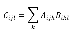
a = torch.randn(3,2,5) b = torch.randn(3,5,3) torch.einsum('ijk,ikl->ijl', [a, b]) |
测试表格
| 字段1 | 字段2 | 字段3 | 字段4 | 字段5 |
|---|---|---|---|---|
| 中国 | python3.8 | tensorflow2 | pytorch1.9 | |
| Row:2 Cell:1 | Row:2 Cell:2 | Row:2 Cell:3 | Row:2 Cell:4 | Row:2 Cell:5 |
| Row:3 Cell:1 | Row:3 Cell:2 | Row:3 Cell:3 | Row:3 Cell:4 | Row:3 Cell:5 |
| Row:4 Cell:1 | Row:4 Cell:2 | Row:4 Cell:3 | Row:4 Cell:4 | Row:4 Cell:5 |
| Row:5 Cell:1 | Row:5 Cell:2 | Row:5 Cell:3 | Row:5 Cell:4 | Row:5 Cell:5 |
| Row:6 Cell:1 | Row:6 Cell:2 | Row:6 Cell:3 | Row:6 Cell:4 | Row:6 Cell:5 |
C.1 einops简介
张量(Tensor)操作是机器学习、深度学习中的常用操作,这些操作在
NumPy、Tensorflow、PyTorch、Mxnet、Paddle等框架都有相应的函数。比如PyTorch中的review,transpose,permute等操作。
einops是提供常用张量操作的Python包,支持NumPy、Tensorflow、PyTorch等框架,可以与这些框架有机衔接。其功能涵盖了reshape、view、transpose和permute等操作。其特点是可读性强、易维护,如变更轴的顺序的操作。
|
1 2 3 4 |
#用传统方法 y = x.transpose(0, 2, 3, 1) #这个功能用einops实现 y = rearrange(x, 'b c h w -> b h w c') |
einops可用pip安装
|
1 |
pip install eniops |
einops的常用函数:rearrange, reduce, repeat
C.1.1 rearrange
rearrange只改变形状,但不改变元素总个数,其功能涵盖transpose, reshape, stack, concatenate, squeeze 和expand_dims等。
1、导入需要的库
|
1 2 3 4 5 6 7 8 9 10 11 12 13 14 15 16 17 18 19 20 21 22 23 24 |
import numpy as np from einops import rearrange, reduce, repeat from PIL.Image import fromarray from IPython import get_ipython #定义一个函数,用于自动可视化arrays数组 def display_np_arrays_as_images(): def np_to_png(a): if 2 <= len(a.shape) <= 3: return fromarray(np.array(np.clip(a, 0, 1) * 255, dtype='uint8'))._repr_png_() else: return fromarray(np.zeros([1, 1], dtype='uint8'))._repr_png_() def np_to_text(obj, p, cycle): if len(obj.shape) < 2: print(repr(obj)) if 2 <= len(obj.shape) <= 3: pass else: print(''.format(obj.shape)) get_ipython().display_formatter.formatters['image/png'].for_type(np.ndarray, np_to_png) get_ipython().display_formatter.formatters['text/plain'].for_type(np.ndarray, np_to_text) |
2、自动可视化arrays数据
|
1 2 |
#把arrays以图像方式显示 display_np_arrays_as_images() |
3、导入测试数据
数据文件下载地址:https://github.com/arogozhnikov/einops/tree/master/docs/resources
|
1 2 3 |
ims = np.load('../data/test_images.npy', allow_pickle=False) # 共有6张图,形状为96x96x3 print(ims.shape, ims.dtype) # (6, 96, 96, 3) float64 |
(1)测试数据
|
1 2 |
#显示第1张图 ims[0] |

(2)显示第2张图
|
1 2 |
#显示第2张图 ims[1] |

4、交互维度
|
1 2 |
##交互宽和高维度 rearrange(ims[0], 'h w c -> w h c') |
5、轴的拼接
涵盖Stack and concatenate等功能。
|
1 2 |
##沿w方向,把原图堆叠成一个3维张量 rearrange(ims, 'b h w c -> h (b w) c') |

6、轴的拆分
(1)拆分batch轴
|
1 2 |
# 把batch=6 分解为b1=2和b2=3,变成一个5维张量 rearrange(ims, '(b1 b2) h w c -> b1 b2 h w c ', b1=2).shape |
(2)拆分与拼接(concatenate)
|
1 2 |
# 同时利用轴的拼接与拆分 rearrange(ims, '(b1 b2) h w c -> (b1 h) (b2 w) c ', b1=2) |

(3)对width轴进行拆分
|
1 2 |
#把一部分width 维度上的值移到height维度上 rearrange(ims, 'b h (w w2) c -> (h w2) (b w) c', w2=2) |

7、重新拼接轴
|
1 |
rearrange(ims, 'b h w c -> h (b w) c') |

8、沿轴增加或减少一个维度
覆盖这些函数的功能:Squeeze and unsqueeze (expand_dims)
|
1 2 3 |
x = rearrange(ims, 'b h w c -> b 1 h w 1 c') # 等价于numpy.expand_dims print(x.shape) print(rearrange(x, 'b 1 h w 1 c -> b h w c').shape) # 等价于 numpy.squeeze |
(6, 1, 96, 96, 1, 3)
(6, 96, 96, 3)
C.1.2 reduce
沿轴求平均值,最大值、最小值等。
|
1 2 3 4 5 |
# 沿batch轴进行平均,等价于ims.mean(axis=0),但reduce可读性更好 reduce(ims, 'b h w c -> h w c', 'mean') # 把图像分成2x2大小的块,然后对每块求平均,其输出形状为:48x(6x48)x3 #也可把mean改为max或min reduce(ims, 'b (h h2) (w w2) c -> h (b w) c', 'mean', h2=2, w2=2) |
C.1.3 repeat
在某轴上重复n次。
|
1 2 |
# 沿width维度重复n次 repeat(ims[0], 'h w c -> h (repeat w) c', repeat=3) |

|
1 2 |
# 沿highth及width维度复制多个元素 repeat(ims[0], 'h w c -> (2 h) (2 w) c') |

C.2 作为pytorch的layer来使用
Rearrange是nn.module的子类,直接可以当作pytorch网络层放到模型里。
C.2.1 展平
|
1 2 3 4 5 6 7 8 9 10 11 12 13 14 15 |
from torch.nn import Sequential, Conv2d, MaxPool2d, Linear, ReLU from einops.layers.torch import Rearrange from einops.layers.torch import Reduce model = Sequential( Conv2d(3, 6, kernel_size=5), MaxPool2d(kernel_size=2), Conv2d(6, 16, kernel_size=5), MaxPool2d(kernel_size=2), #展平 Rearrange('b c h w -> b (c h w)'), Linear(16*5*5, 120), ReLU(), Linear(120, 10), ) |
这个代码与下代码等价
|
1 2 3 4 5 6 7 8 9 10 |
model01 = Sequential( Conv2d(3, 6, kernel_size=5), MaxPool2d(kernel_size=2), Conv2d(6, 16, kernel_size=5), #最大池化并展平 Reduce('b c (h 2) (w 2) -> b (c h w)', 'max'), Linear(16*5*5, 120), ReLU(), Linear(120, 10), ) |
C.2.2 使用einops可大大简化PyTorch代码
1、构建模型
|
1 2 3 4 5 6 7 8 9 10 11 12 13 14 15 16 17 18 19 20 21 22 23 24 25 26 27 28 |
import torch import torch.nn as nn import torch.nn.functional as F import numpy as np import math from einops import rearrange, reduce, asnumpy, parse_shape from einops.layers.torch import Rearrange, Reduce class Net(nn.Module): def __init__(self): super(Net, self).__init__() self.conv1 = nn.Conv2d(1, 10, kernel_size=5) self.conv2 = nn.Conv2d(10, 20, kernel_size=5) self.conv2_drop = nn.Dropout2d() self.fc1 = nn.Linear(320, 50) self.fc2 = nn.Linear(50, 10) def forward(self, x): x = F.relu(F.max_pool2d(self.conv1(x), 2)) x = F.relu(F.max_pool2d(self.conv2_drop(self.conv2(x)), 2)) x = x.view(-1, 320) x = F.relu(self.fc1(x)) x = F.dropout(x, training=self.training) x = self.fc2(x) return F.log_softmax(x, dim=1) conv_net_old = Net() |
2、代码1与下面这个代码等价
|
1 2 3 4 5 6 7 8 9 10 11 12 13 14 15 |
conv_net_new = nn.Sequential( nn.Conv2d(1, 10, kernel_size=5), nn.MaxPool2d(kernel_size=2), nn.ReLU(), nn.Conv2d(10, 20, kernel_size=5), nn.MaxPool2d(kernel_size=2), nn.ReLU(), nn.Dropout2d(), Rearrange('b c h w -> b (c h w)'), nn.Linear(320, 50), nn.ReLU(), nn.Dropout(), nn.Linear(50, 10), nn.LogSoftmax(dim=1) ) |
C.2.3 构建注意力模型
|
1 2 3 4 5 6 7 8 9 |
class Attention(nn.Module): def __init__(self): super(Attention, self).__init__() def forward(self, K, V, Q): A = torch.bmm(K.transpose(1,2), Q) / np.sqrt(Q.shape[1]) A = F.softmax(A, 1) R = torch.bmm(V, A) return torch.cat((R, Q), dim=1) |
这段代码与下列代码等价
|
1 2 3 4 5 6 |
def attention(K, V, Q): _, n_channels, _ = K.shape A = torch.einsum('bct,bcl->btl', [K, Q]) A = F.softmax(A * n_channels ** (-0.5), 1) R = torch.einsum('bct,btl->bcl', [V, A]) return torch.cat((R, Q), dim=1) |
1.自注意力(Self-Attention)
Transformer凭借其自注意力机制,有效解决了字符之间或像素之间的长距离依赖,日益称为NLP和CV领域的通用架构。
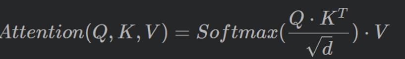
自注意力机制是Transformer的核心,如何简洁有效实现Self-Attention?这里介绍一种法,使用einops和PyTorch中einsum。自注意力的计算公式如下
2.自注意力计算的详细过程如下图所示
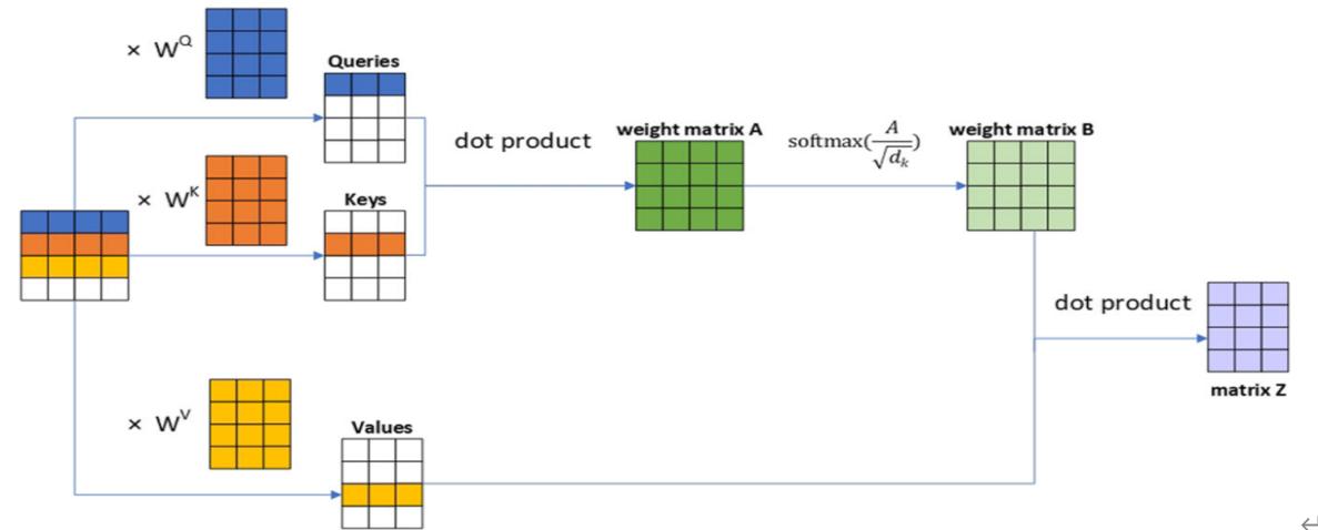
这里假设x的形状(1,4,4),标记(Token)个数为4,每个token转换为长度为4的向量,嵌入(Embedding)的维度为3(dim=3)。
3、详细实现代码
用代码实现上述计算过程
|
1 2 3 4 5 6 7 8 9 10 11 12 13 14 15 16 17 18 19 20 21 22 23 24 25 26 27 28 29 30 31 32 33 34 35 36 37 38 39 40 41 42 |
import numpy as np import torch from einops import rearrange from torch import nn class SelfAttentionAISummer(nn.Module): """ 使用einsum生成自注意力 """ def __init__(self, dim): """ 参数说明: dim: 嵌入向量(embedding vector)维度 输入x假设为3D向量(如b,h,w) """ super().__init__() # 利用全连接层生成Q,K,V这3个4x3矩阵 self.to_qvk = nn.Linear(4, dim * 3, bias=False) # 得到dim(即d)的根号的倒数值 self.scale_factor = dim ** -0.5 # 1/np.sqrt(dim) def forward(self, x, mask=None): assert x.dim() == 3, '3D tensor must be provided' # 生成qkv qkv = self.to_qvk(x) # [batch, tokens, dim*3 ] # 把qkv拆分成q,v,k # rearrange tensor to [3, batch, tokens, dim] and cast to tuple q, k, v = tuple(rearrange(qkv, 'b t (d k) -> k b t d ', k=3)) # 生成结果的形状为: [batch, tokens, tokens] scaled_dot_prod = torch.einsum('b i d , b j d -> b i j', q, k) * self.scale_factor if mask is not None: assert mask.shape == scaled_dot_prod.shape[1:] scaled_dot_prod = scaled_dot_prod.masked_fill(mask, -np.inf) attention = torch.softmax(scaled_dot_prod, dim=-1) #返回查询Q对各关键字的权重(即attention)与V相乘的结果 return torch.einsum('b i j , b j d -> b i d', attention, v) |
4、测试
|
1 2 3 4 5 |
#输入dim=3 attention=SelfAttentionAISummer(3) #假设输入x为1x4x4矩阵(共4个token) x = torch.rand(1,4,4) attention(x) |
运行结果
tensor([[[-0.3127, 0.4551, -0.0695],
[-0.3176, 0.4594, -0.0715],
[-0.3133, 0.4551, -0.0703],
[-0.3116, 0.4531, -0.0702]]], grad_fn=)
einops的使用可参考官网:
https://github.com/arogozhnikov/einops
使用Swin-Transformer模型实现分类任务
最近几年,Transformer体系结构已成为自然语言处理任务的实际标准,
但其在计算机视觉中的应用还受到限制。在视觉上,注意力要么与卷积网络结合使用,
要么用于替换卷积网络的某些组件,同时将其整体结构保持在适当的位置。2020年10月22日,谷歌人工智能研究院发表一篇题为“An Image is Worth 16x16 Words: Transformers for Image Recognition at Scale”的文章。文章将图像切割成一个个图像块,组成序列化的数据输入Transformer执行图像分类任务。当对大量数据进行预训练并将其传输到多个中型或小型图像识别数据集(如ImageNet、CIFAR-100、VTAB等)时,与目前的卷积网络相比,Vision Transformer(ViT)获得了出色的结果,同时所需的计算资源也大大减少。
2021年3月 微软亚洲研究院 发表的论文《Swin Transformer: Hierarchical Vision Transformer using Shifted Windows》被评为ICCV 2021 最佳论文!
论文地址:https://arxiv.org/pdf/2103.14030.pdf
项目地址:https://github.com/microsoft/Swin-Transformer
这篇论文的作者主要包括中国科学技术大学的刘泽、西安交通大学的林宇桐、微软的曹越和胡瀚等人。该研究提出了一种新的 vision Transformer,即 Swin Transformer,它可以作为计算机视觉的通用骨干(Backbone)。在CV各应用领域,如分类、目标检测、语义分割、实例分割等都超过基于CNN的网络性能!人们自然会问,为啥能取得如此好的效果?为什么ViT没有取得这么好的成绩?
第一个问题:
因为Swin Transformer吸收了Transformer的固有优点(如通用性强、并发处理、超长视野等优点,如图1-1所示),同时吸收了CNN的平移不变性、局部性、层次性等优点。
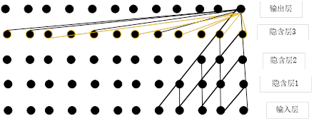
图1-1 卷积神经网络、Transformer架构像素之间的关系
卷积神经网络输出一个像素与输入5个像素点之间建立联系需要经过3个隐含层;而Transformer中输出一个像素点与其他每个像素点建立联系只要一层就可以。
第二个问题:
ViT的计算复杂度没有降低,ViT结构没有层次。如1-2所示:
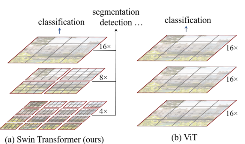
图1-2 Swin Transformer 与ViT层级结构的异同
Swin Transformer是如何实现这些优点的呢?
1、降低计算复杂度:采用局部性,如图1-2所示,把特征图·划分为不重叠的不同尺寸的窗口,计算自注意力时只在这些窗口内。
2、计算在窗口内,但通过窗口shifted方法,可以把相邻窗口的信息连接起来,如图1-3所示。

图1-3 Swin Transformer中windows shifted 的示意图
通过Windows shifted后的多头注意力计算简称为SW-MSA的具体计算,window
内的多头注意力计算简称为W-MSA,具体位置可参考图1-4。
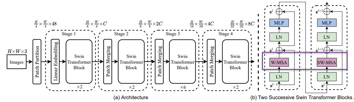
图1-4 Swin Transformer的架构图
这里我们以Swin Transformer为模型,实现对数据CiFar10的分类工作,模型性能得到进一步的提升。以下为用swin-transformer架构实现一个分类任务的详细代码。
1、导入模型
|
1 2 3 4 5 6 7 8 9 10 |
import os import math import numpy as np import pickle as p import tensorflow as tf from tensorflow import keras import matplotlib.pyplot as plt import tensorflow_addons as tfa from tensorflow.keras import layers %matplotlib inline |
这里使用了TensorFlow_addons模块,它实现了核心 TensorFlow 中未提供的新功能。
tensorflow_addons的安装要注意与tf的版本对应关系,请参考:
https://github.com/tensorflow/addons。
安装addons时要注意其版本与tensorflow版本的对应,具体关系以上这个链接有。
2、定义加载函数
|
1 2 3 4 5 6 7 8 9 10 11 12 13 14 15 16 17 18 19 20 21 |
def load_CIFAR_data(data_dir): """load CIFAR data""" images_train=[] labels_train=[] for i in range(5): f=os.path.join(data_dir,'data_batch_%d' % (i+1)) print('loading ',f) # 调用 load_CIFAR_batch( )获得批量的图像及其对应的标签 image_batch,label_batch=load_CIFAR_batch(f) images_train.append(image_batch) labels_train.append(label_batch) Xtrain=np.concatenate(images_train) Ytrain=np.concatenate(labels_train) del image_batch ,label_batch Xtest,Ytest=load_CIFAR_batch(os.path.join(data_dir,'test_batch')) print('finished loadding CIFAR-10 data') # 返回训练集的图像和标签,测试集的图像和标签 return (Xtrain,Ytrain),(Xtest,Ytest) |
3、定义批量加载函数
|
1 2 3 4 5 6 7 8 9 10 11 12 13 14 15 16 17 18 19 20 |
def load_CIFAR_batch(filename): """ load single batch of cifar """ with open(filename, 'rb')as f: # 一个样本由标签和图像数据组成 # (3072=32x32x3) # ... # data_dict = p.load(f, encoding='bytes') images= data_dict[b'data'] labels = data_dict[b'labels'] # 把原始数据结构调整为: BCWH images = images.reshape(10000, 3, 32, 32) # tensorflow处理图像数据的结构:BWHC # 把通道数据C移动到最后一个维度 images = images.transpose (0,2,3,1) labels = np.array(labels) return images, labels |
4、加载数据
|
1 2 |
data_dir = '../data/cifar-10-batches-py' (x_train,y_train),(x_test,y_test) = load_CIFAR_data(data_dir) |
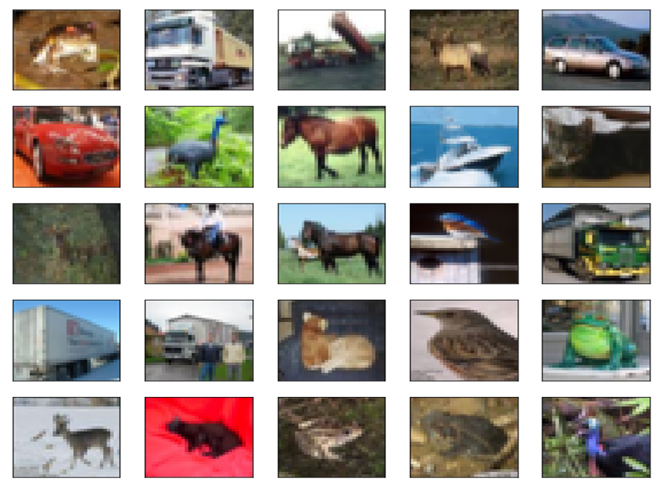
5、定义数据预处理及训练模型的一些超参数
|
1 2 3 4 5 6 7 8 9 10 11 12 13 14 15 16 17 |
num_classes = 10 input_shape = (32, 32, 3) x_train, x_test = x_train / 255.0, x_test / 255.0 y_train = keras.utils.to_categorical(y_train, num_classes) y_test = keras.utils.to_categorical(y_test, num_classes) print(f"x_train shape: {x_train.shape} - y_train shape: {y_train.shape}") print(f"x_test shape: {x_test.shape} - y_test shape: {y_test.shape}") plt.figure(figsize=(10, 10)) for i in range(25): plt.subplot(5, 5, i + 1) plt.xticks([]) plt.yticks([]) plt.grid(False) plt.imshow(x_train[i]) plt.show() |
6、设置一些超参数
|
1 2 3 4 5 6 7 8 9 10 11 12 13 14 15 16 17 18 19 |
patch_size = (2, 2) # 2-by-2 sized patches dropout_rate = 0.03 # Dropout rate num_heads = 8 # Attention heads embed_dim = 64 # Embedding dimension num_mlp = 256 # MLP layer size qkv_bias = True # Convert embedded patches to query, key, and values with a learnable additive value window_size = 2 # Size of attention window shift_size = 1 # Size of shifting window image_dimension = 32 # Initial image size num_patch_x = input_shape[0] // patch_size[0] num_patch_y = input_shape[1] // patch_size[1] learning_rate = 1e-3 batch_size = 128 num_epochs = 100 validation_split = 0.1 weight_decay = 0.0001 label_smoothing = 0.1 |
7、定义几个辅助函数
|
1 2 3 4 5 6 7 8 9 10 11 12 13 14 15 16 17 18 19 20 21 22 23 24 25 26 27 28 29 30 31 32 33 34 35 36 37 38 |
def window_partition(x, window_size): _, height, width, channels = x.shape patch_num_y = height // window_size patch_num_x = width // window_size x = tf.reshape( x, shape=(-1, patch_num_y, window_size, patch_num_x, window_size, channels) ) x = tf.transpose(x, (0, 1, 3, 2, 4, 5)) windows = tf.reshape(x, shape=(-1, window_size, window_size, channels)) return windows def window_reverse(windows, window_size, height, width, channels): patch_num_y = height // window_size patch_num_x = width // window_size x = tf.reshape( windows, shape=(-1, patch_num_y, patch_num_x, window_size, window_size, channels), ) x = tf.transpose(x, perm=(0, 1, 3, 2, 4, 5)) x = tf.reshape(x, shape=(-1, height, width, channels)) return x class DropPath(layers.Layer): def __init__(self, drop_prob=None, **kwargs): super(DropPath, self).__init__(**kwargs) self.drop_prob = drop_prob def call(self, x): input_shape = tf.shape(x) batch_size = input_shape[0] rank = x.shape.rank shape = (batch_size,) + (1,) * (rank - 1) random_tensor = (1 - self.drop_prob) + tf.random.uniform(shape, dtype=x.dtype) path_mask = tf.floor(random_tensor) output = tf.math.divide(x, 1 - self.drop_prob) * path_mask return output |
8、 定义W-MSA类
|
1 2 3 4 5 6 7 8 9 10 11 12 13 14 15 16 17 18 19 20 21 22 23 24 25 26 27 28 29 30 31 32 33 34 35 36 37 38 39 40 41 42 43 44 45 46 47 48 49 50 51 52 53 54 55 56 57 58 59 60 61 62 63 64 65 66 67 68 69 70 71 72 73 74 75 76 77 78 79 80 81 82 83 |
class WindowAttention(layers.Layer): def __init__( self, dim, window_size, num_heads, qkv_bias=True, dropout_rate=0.0, **kwargs ): super(WindowAttention, self).__init__(**kwargs) self.dim = dim self.window_size = window_size self.num_heads = num_heads self.scale = (dim // num_heads) ** -0.5 self.qkv = layers.Dense(dim * 3, use_bias=qkv_bias) self.dropout = layers.Dropout(dropout_rate) self.proj = layers.Dense(dim) def build(self, input_shape): num_window_elements = (2 * self.window_size[0] - 1) * ( 2 * self.window_size[1] - 1 ) self.relative_position_bias_table = self.add_weight( shape=(num_window_elements, self.num_heads), initializer=tf.initializers.Zeros(), trainable=True, ) coords_h = np.arange(self.window_size[0]) coords_w = np.arange(self.window_size[1]) coords_matrix = np.meshgrid(coords_h, coords_w, indexing="ij") coords = np.stack(coords_matrix) coords_flatten = coords.reshape(2, -1) relative_coords = coords_flatten[:, :, None] - coords_flatten[:, None, :] relative_coords = relative_coords.transpose([1, 2, 0]) relative_coords[:, :, 0] += self.window_size[0] - 1 relative_coords[:, :, 1] += self.window_size[1] - 1 relative_coords[:, :, 0] *= 2 * self.window_size[1] - 1 relative_position_index = relative_coords.sum(-1) self.relative_position_index = tf.Variable( initial_value=tf.convert_to_tensor(relative_position_index), trainable=False ) def call(self, x, mask=None): _, size, channels = x.shape head_dim = channels // self.num_heads x_qkv = self.qkv(x) x_qkv = tf.reshape(x_qkv, shape=(-1, size, 3, self.num_heads, head_dim)) x_qkv = tf.transpose(x_qkv, perm=(2, 0, 3, 1, 4)) q, k, v = x_qkv[0], x_qkv[1], x_qkv[2] q = q * self.scale k = tf.transpose(k, perm=(0, 1, 3, 2)) attn = q @ k num_window_elements = self.window_size[0] * self.window_size[1] relative_position_index_flat = tf.reshape( self.relative_position_index, shape=(-1,) ) relative_position_bias = tf.gather( self.relative_position_bias_table, relative_position_index_flat ) relative_position_bias = tf.reshape( relative_position_bias, shape=(num_window_elements, num_window_elements, -1) ) relative_position_bias = tf.transpose(relative_position_bias, perm=(2, 0, 1)) attn = attn + tf.expand_dims(relative_position_bias, axis=0) if mask is not None: nW = mask.get_shape()[0] mask_float = tf.cast( tf.expand_dims(tf.expand_dims(mask, axis=1), axis=0), tf.float32 ) attn = ( tf.reshape(attn, shape=(-1, nW, self.num_heads, size, size)) + mask_float ) attn = tf.reshape(attn, shape=(-1, self.num_heads, size, size)) attn = keras.activations.softmax(attn, axis=-1) else: attn = keras.activations.softmax(attn, axis=-1) attn = self.dropout(attn) x_qkv = attn @ v x_qkv = tf.transpose(x_qkv, perm=(0, 2, 1, 3)) x_qkv = tf.reshape(x_qkv, shape=(-1, size, channels)) x_qkv = self.proj(x_qkv) x_qkv = self.dropout(x_qkv) return x_qkv |
9、定义SwinTransformer 模块
|
1 2 3 4 5 6 7 8 9 10 11 12 13 14 15 16 17 18 19 20 21 22 23 24 25 26 27 28 29 30 31 32 33 34 35 36 37 38 39 40 41 42 43 44 45 46 47 48 49 50 51 52 53 54 55 56 57 58 59 60 61 62 63 64 65 66 67 68 69 70 71 72 73 74 75 76 77 78 |
class SwinTransformer(layers.Layer): def __init__( self, dim, num_patch, num_heads, window_size=7, shift_size=0, num_mlp=1024, qkv_bias=True, dropout_rate=0.0, **kwargs, ): super(SwinTransformer, self).__init__(**kwargs) self.dim = dim # number of input dimensions self.num_patch = num_patch # number of embedded patches self.num_heads = num_heads # number of attention heads self.window_size = window_size # size of window self.shift_size = shift_size # size of window shift self.num_mlp = num_mlp # number of MLP nodes self.norm1 = layers.LayerNormalization(epsilon=1e-5) self.attn = WindowAttention( dim, window_size=(self.window_size, self.window_size), num_heads=num_heads, qkv_bias=qkv_bias, dropout_rate=dropout_rate, ) self.drop_path = DropPath(dropout_rate) self.norm2 = layers.LayerNormalization(epsilon=1e-5) self.mlp = keras.Sequential( [ layers.Dense(num_mlp), layers.Activation(keras.activations.gelu), layers.Dropout(dropout_rate), layers.Dense(dim), layers.Dropout(dropout_rate), ] ) if min(self.num_patch) < self.window_size: self.shift_size = 0 self.window_size = min(self.num_patch) def build(self, input_shape): if self.shift_size == 0: self.attn_mask = None else: height, width = self.num_patch h_slices = ( slice(0, -self.window_size), slice(-self.window_size, -self.shift_size), slice(-self.shift_size, None), ) w_slices = ( slice(0, -self.window_size), slice(-self.window_size, -self.shift_size), slice(-self.shift_size, None), ) mask_array = np.zeros((1, height, width, 1)) count = 0 for h in h_slices: for w in w_slices: mask_array[:, h, w, :] = count count += 1 mask_array = tf.convert_to_tensor(mask_array) # mask array to windows mask_windows = window_partition(mask_array, self.window_size) mask_windows = tf.reshape( mask_windows, shape=[-1, self.window_size * self.window_size] ) attn_mask = tf.expand_dims(mask_windows, axis=1) - tf.expand_dims( mask_windows, axis=2 ) attn_mask = tf.where(attn_mask != 0, -100.0, attn_mask) attn_mask = tf.where(attn_mask == 0, 0.0, attn_mask) self.attn_mask = tf.Variable(initial_value=attn_mask, trainable=False) def call(self, x): height, width = self.num_patch _, num_patches_before, channels = x.shape x_skip = x x = self.norm1(x) x = tf.reshape(x, shape=(-1, height, width, channels)) if self.shift_size > 0: shifted_x = tf.roll( x, shift=[-self.shift_size, -self.shift_size], axis=[1, 2] ) else: shifted_x = x x_windows = window_partition(shifted_x, self.window_size) x_windows = tf.reshape( x_windows, shape=(-1, self.window_size * self.window_size, channels) ) attn_windows = self.attn(x_windows, mask=self.attn_mask) attn_windows = tf.reshape( attn_windows, shape=(-1, self.window_size, self.window_size, channels) ) shifted_x = window_reverse( attn_windows, self.window_size, height, width, channels ) if self.shift_size > 0: x = tf.roll( shifted_x, shift=[self.shift_size, self.shift_size], axis=[1, 2] ) else: x = shifted_x x = tf.reshape(x, shape=(-1, height * width, channels)) x = self.drop_path(x) x = x_skip + x x_skip = x x = self.norm2(x) x = self.mlp(x) x = self.drop_path(x) x = x_skip + x return x |
10、抽取特征
|
1 2 3 4 5 6 7 8 9 10 11 12 13 14 15 16 17 18 19 20 21 22 23 24 25 26 27 28 29 30 31 32 33 34 35 36 37 38 39 40 41 42 43 44 45 46 47 48 49 50 |
class PatchExtract(layers.Layer): def __init__(self, patch_size, **kwargs): super(PatchExtract, self).__init__(**kwargs) self.patch_size_x = patch_size[0] self.patch_size_y = patch_size[0] def call(self, images): batch_size = tf.shape(images)[0] patches = tf.image.extract_patches( images=images, sizes=(1, self.patch_size_x, self.patch_size_y, 1), strides=(1, self.patch_size_x, self.patch_size_y, 1), rates=(1, 1, 1, 1), padding="VALID", ) patch_dim = patches.shape[-1] patch_num = patches.shape[1] return tf.reshape(patches, (batch_size, patch_num * patch_num, patch_dim)) class PatchEmbedding(layers.Layer): def __init__(self, num_patch, embed_dim, **kwargs): super(PatchEmbedding, self).__init__(**kwargs) self.num_patch = num_patch self.proj = layers.Dense(embed_dim) self.pos_embed = layers.Embedding(input_dim=num_patch, output_dim=embed_dim) def call(self, patch): pos = tf.range(start=0, limit=self.num_patch, delta=1) return self.proj(patch) + self.pos_embed(pos) class PatchMerging(tf.keras.layers.Layer): def __init__(self, num_patch, embed_dim): super(PatchMerging, self).__init__() self.num_patch = num_patch self.embed_dim = embed_dim self.linear_trans = layers.Dense(2 * embed_dim, use_bias=False) def call(self, x): height, width = self.num_patch _, _, C = x.get_shape().as_list() x = tf.reshape(x, shape=(-1, height, width, C)) x0 = x[:, 0::2, 0::2, :] x1 = x[:, 1::2, 0::2, :] x2 = x[:, 0::2, 1::2, :] x3 = x[:, 1::2, 1::2, :] x = tf.concat((x0, x1, x2, x3), axis=-1) x = tf.reshape(x, shape=(-1, (height // 2) * (width // 2), 4 * C)) return self.linear_trans(x) |
11、构建模型
|
1 2 3 4 5 6 7 8 9 10 11 12 13 14 15 16 17 18 19 20 21 22 23 24 25 26 27 28 |
input = layers.Input(input_shape) x = layers.experimental.preprocessing.RandomCrop(image_dimension, image_dimension)(input) x = layers.experimental.preprocessing.RandomFlip("horizontal")(x) x = PatchExtract(patch_size)(x) x = PatchEmbedding(num_patch_x * num_patch_y, embed_dim)(x) x = SwinTransformer( dim=embed_dim, num_patch=(num_patch_x, num_patch_y), num_heads=num_heads, window_size=window_size, shift_size=0, num_mlp=num_mlp, qkv_bias=qkv_bias, dropout_rate=dropout_rate, )(x) x = SwinTransformer( dim=embed_dim, num_patch=(num_patch_x, num_patch_y), num_heads=num_heads, window_size=window_size, shift_size=shift_size, num_mlp=num_mlp, qkv_bias=qkv_bias, dropout_rate=dropout_rate, )(x) x = PatchMerging((num_patch_x, num_patch_y), embed_dim=embed_dim)(x) x = layers.GlobalAveragePooling1D()(x) output = layers.Dense(num_classes, activation="softmax")(x) |
12、训练模型
|
1 2 3 4 5 6 7 8 9 10 11 12 13 14 15 16 17 18 19 |
model = keras.Model(input, output) model.compile( loss=keras.losses.CategoricalCrossentropy(label_smoothing=label_smoothing), optimizer=tfa.optimizers.AdamW( learning_rate=learning_rate, weight_decay=weight_decay ), metrics=[ keras.metrics.CategoricalAccuracy(name="accuracy"), keras.metrics.TopKCategoricalAccuracy(5, name="top-5-accuracy"), ], ) history = model.fit( x_train, y_train, batch_size=batch_size, epochs=num_epochs, validation_split=validation_split, ) |
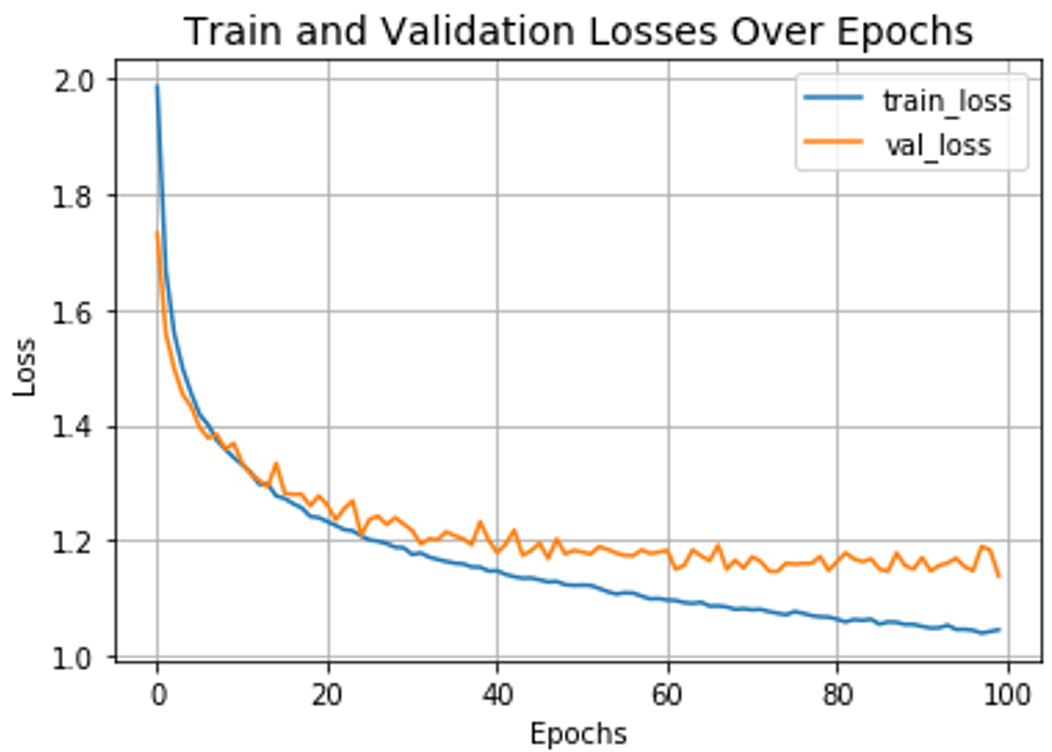
13、可视化运行结果
|
1 2 3 4 5 6 7 8 |
plt.plot(history.history["loss"], label="train_loss") plt.plot(history.history["val_loss"], label="val_loss") plt.xlabel("Epochs") plt.ylabel("Loss") plt.title("Train and Validation Losses Over Epochs", fontsize=14) plt.legend() plt.grid() plt.show() |
运行结果
14、测试结果
|
1 2 3 4 |
loss, accuracy, top_5_accuracy = model.evaluate(x_test, y_test) print(f"Test loss: {round(loss, 2)}") print(f"Test accuracy: {round(accuracy * 100, 2)}%") print(f"Test top 5 accuracy: {round(top_5_accuracy * 100, 2)}%") |
15、可视化测试结果
|
1 2 3 4 5 6 7 8 9 |
plt.plot(history.history["accuracy"], label="train_accuracy") plt.plot(history.history["val_accuracy"], label="val_accuracy") plt.plot(history.history["val_top-5-accuracy"], label="val_top5_accuracy") plt.xlabel("Epochs") plt.ylabel("Loss") plt.title("Train and Validation Losses Over Epochs", fontsize=14) plt.legend() plt.grid() plt.show() |

1、元宇宙
本质上,我认为元宇宙是AR、VR眼镜上的整个互联网,是互联网在新计算平台上的一种呈现方式。”

谭平认为,过去我们经历了计算平台从PC向智能手机的转变,许多互联网应用因此而改变,比如PC上的社交有QQ和MSN,到了手机上就全变成微信。电商也经历了类似的变化——比如在手机时代,电商领域出现了本地生活,因为智能手机能够提供用户的定位,所以可以给用户推荐三公里以内的优质服务,“这在PC时代是无法做到的,这是新平台的新特性带来的新用户体验。”
2021年,元宇宙成为一个让所有科技公司蠢蠢欲动的关键词,但讨论至今,它究竟代表了什么还没有明确的定义。
在谭平看来,元宇宙的范畴非常广泛,包括社交、电商、游戏、教育,甚至是支付。“我们今天熟悉的互联网应用,都会在元宇宙时代有新的演变。”
谭平认为,要理解元宇宙对互联网应用带来的变化,就得来看一看VR、AR眼镜的技术本质——新显示和新交互。

他进一步解释称,在过去,不论是PC还是手机,显示界面是两维的,应用程序是一个窗口,我们可以在窗口内点击鼠标、波段等两维的操作;而VR和AR眼镜下的显示界面是三维的,我们会沉浸在一个虚拟的三维信息世界之中,可以通过肢体动作和这个三维世界进行交互。“显示和交互是应用的最底层,这两者的巨变将会引起上层互联网应用的革命。”
基于上述理解,实现“元宇宙”需要的技术也愈发清晰。
2、元宇宙的4大技术层
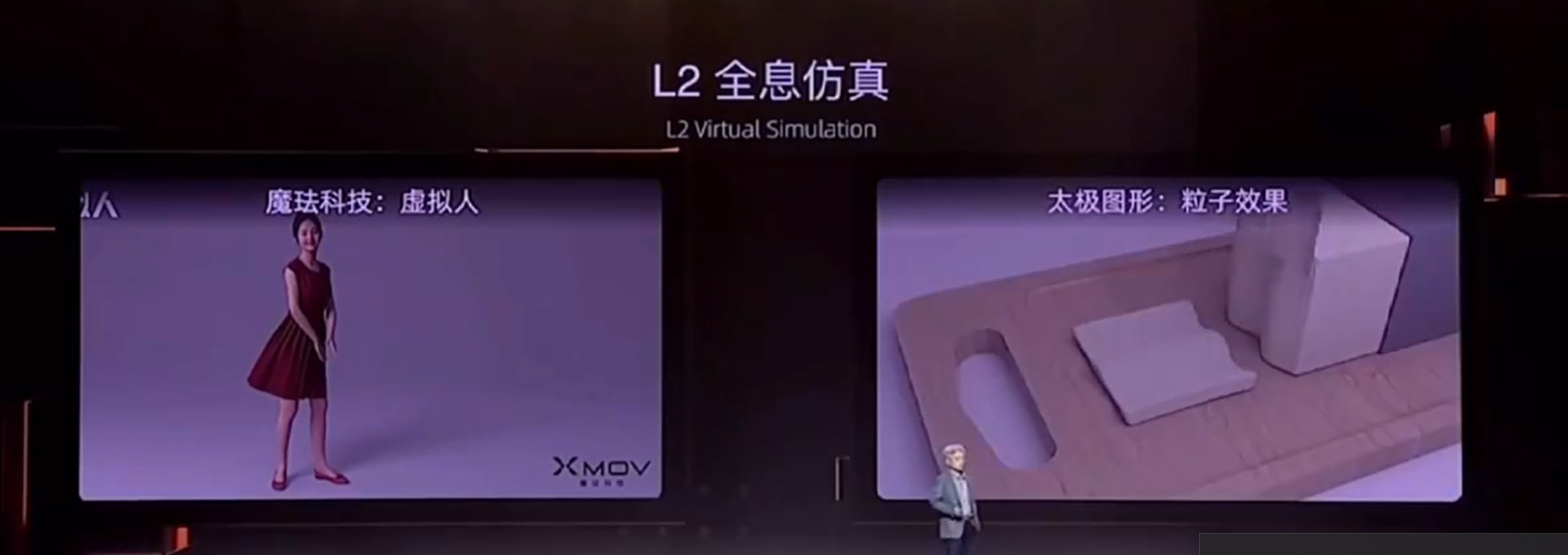
关于元宇宙的技术构成,谭平的看法是,元宇宙的第一层技术是全息构建;第二层是全息仿真;第三层是虚实融合;第四层则是虚实联动。

2.1 全息构建
其中,第一个层面需要构建出整个虚拟世界的几何模型,例如目前的VR看房、看店这样的应用基本上就是这一层,如下图所示。

2.2全息仿真
第二层是全息仿真,这需要构建出虚拟世界的动态过程,让虚拟世界无限逼近真实世界。“比如虚拟世界里的水要能往低处流,扔一块石头要能打碎玻璃,虚拟世界里的角色要能对外界环境作出合理的反应,就像最近的电影《失控玩家》里那样。”
2.3虚实融合
第三层则是虚实融合。谭平介绍称,解决了第一层和第二层的问题,我们就能够构建出一个完美的VR世界,而第三层技术需要让虚拟世界和真实世界融合——实现这一点需要建立真实世界的高清三维地图,并且在地图里做到高精准的定位以及准确地叠加虚拟信息。

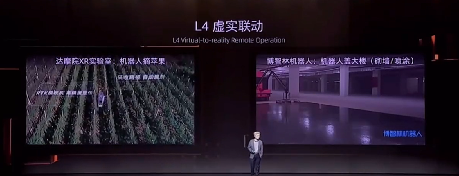
2.4虚实联动
除此之外,最后一个重要的层面是虚实联动,“本质上就是要解决机器人操纵的问题”。谭平称,这通常不在元宇宙的概念中,更多的是他个人的理解:他认为,如果没有这一层,一切的美好只能停留在虚拟世界,而真实世界有可能一塌糊涂,“这并不是我们想要的一个结果。”
3、用元宇宙打造的一个全新的互联网时代即将到来

谭平谈元宇宙的视频:
https://www.zhihu.com/zvideo/1435216634370158592
1.项目概述
运行环境tensorflow2.x,使用VOC2007数据集实现Faster-RCNN目标检测算法。 本文将详细介绍并讲解算法的每个模块和每个函数的功能,并可视化一张图片在训练和测试过程中 的变化情况。 Faster RCNN首次提出了anchor机制,后续大量流行的SSD、R-CNN、Fast RCNN、Faster RCNN、Mask RCNN和RetinaNet等等 模型都是在建立在anchor基础上的,而yolov3、yolov5等模型尽管对anchor做了一些调整,但出发点不变, 都是从anchor的三个任务和参数化坐标出发,因此,Faster RCNN很重要。
本项目基于2.4+版本的tensorflow,使用VOC2007数据集实现Faster-RCNN目标检测算法。接下来将详细讲解Faster-RCNN算法的每个模块的主要功能,期间通过可视化一张图片在训练和测试过程中如何变化的。
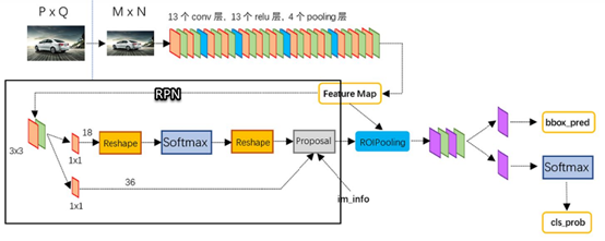
整个Faster-RCNN算法的网络架构图
2.数据描述
VOC2007数据集的结构如下:

各个目录含义如下:
1、Annotations中存储的是.xml文件,即标注数据,标注了影像中的目标类型以及边界框bbox;
2、ImageSet中存储的都是一些txt文件,其实就是各个挑战任务所使用的图片序号,VOC比赛是将所有的图片存在一起,然后不同的挑战任务使用的图片就用一个txt存储使用图片的文件名即可;
3、JPEGImages文件夹中存储了数据集的所有图片;
4、SegmentationClass存储了类别分割的标注png。
5、SegmentationObject存储了实例分割的标注png。 其中类别分割与实例分割的区别是类别分割只区分物体的类别,同样类别的两个不同物体的像素分配同一个值;而实例分割不只区分目标的类别,而且同样类别的两个不同的对象,也要进行区分。例如两个人,在类别分割中都标注为person,而实例分割就需要分割为person1、person2.
VOC2007数据集的更大介绍可参考:https://www.codenong.com/cs106063597/
3.项目流程
1.导入需要的模块
2.导入数据
3.提取特征
4.恢复模型权重参数
5.可视化训练后的特征图
6.实现RPN网络
7.实现RoI Pooling
8.可视化最后结果
3.1 导入需要的模块
|
1 2 3 4 5 6 7 8 9 10 11 12 |
from utils.config import Config from model.fasterrcnn import FasterRCNNTrainer, FasterRCNN from model.fasterrcnn import _fast_rcnn_loc_loss import tensorflow as tf import numpy as np from utils.data import Dataset from utils.nms import nms import matplotlib.pyplot as plt %matplotlib inline |
3.2 导入数据
|
1 2 3 4 5 6 7 8 |
#导入VOC2007数据集 dataset = Dataset(config) #获取数据集中第11张图片和对应的标签 img, bboxes, labels, scale = dataset[11] for x in (img, bboxes, labels): print('shape:', x.shape, 'max:', tf.reduce_max(x).numpy(), 'min:', tf.reduce_min(x).numpy()) print(scale) |
第11张图片基本信息说明:
1、img的shape为(1, 600, 900, 3)分别代表了batch维度,图片的高和宽,通道数;
2、bboxes的类别数及坐标信息,shape为(n, 4),这里n表示该图片所含的类别总数,最大为20,不包括背景;
3、labels的shape为(n,),该图片所含的类别总数,类别代码,这里6表示汽车。
|
1 2 3 4 5 6 7 8 9 10 |
#数据集中20中类别 VOC_BBOX_LABEL_NAMES = ( 'aeroplane', 'bicycle', 'bird', 'boat', 'bottle', 'bus', 'car', 'cat', 'chair', 'cow', 'diningtable', 'dog', 'horse', 'motorbike', 'person', 'pottedplant', 'sheep', 'sofa', 'train', 'tvmonitor') #可视化原图及标注等信息 from utils.data import vis #可视化图片及目标位置 vis(img[0], bboxes, labels) |
运行结果:

3.3 特征提取
这里使用VGG16作为主干网络(backbone),经过backbone之后,输出为特征图,其形状为(1, 38, 57, 512),1代表batch size,38和57代表特征图的高度和宽度,数值上为原来(600, 900)的1/16(中间会有向下取整操作),512代表通道数。
|
1 2 3 4 5 6 7 8 9 10 11 12 13 14 15 16 17 18 |
import datetime from utils.config import Config from model.fasterrcnn import FasterRCNNTrainer, FasterRCNN import tensorflow as tf from utils.data import Dataset physical_devices = tf.config.experimental.list_physical_devices('GPU') assert len(physical_devices) > 0, "Not enough GPU hardware devices available" tf.config.experimental.set_memory_growth(physical_devices[0], True) config = Config() config._parse({}) print("读取数据中....") dataset = Dataset(config) frcnn = FasterRCNN(21, (7, 7)) print('model construct completed') |
待续……
一、目标检测的目的和挑战
1、目标检测的目的
目标检测的目的是什么?主要就是:
(1)确定目标对象所在位置及大小;
(2)确定目标对象的类别
第1点是属于检测,第2点识别,重点是检测,目标图像检测后识别与一般图像识别一样。如何检测目标对象?我们可以通过以下图像更形象地进行说明。为简便起见,我们假设图像中只有1个目标对象(或少数几个目标对象),对这个图像进行检测的目标就是,
用矩形框界定目标对象,如下图所示。
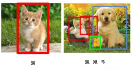
图1 目标检测示意图
把要检测的目标用矩阵图框定,然后对框定的目标进行分类,这就是目标检测的主要目标。框定目标并识别目标两个任务中,框定目标是关键。如何框定目标呢?
我们从简单的情况开始,然后,再考虑更复杂的情况。
假设图像中只有一个目标,如图1的左图。这种情况,我们凭直觉最先想到的或许就是使用一个矩形框窗口,从左到右移动,如图2所示。

图2 用一个框进行自左向右移动示意图
这是一种非常理想情况,使用的框大小正好能框,这些候选框确定后,就可以针对每个框使用分类模型计算各框为猫的概率或得分,如图3所示。看哪个框的得分最高就选择哪个框,从图3 可知,中间这个框内容对象为猫的概率最大,故选择这个框(如图1左图所示)。框确定意味着这个框的左上点的坐标(x,y)及这个框的高(h)和宽(w)也确定了。
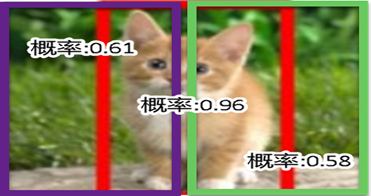
图3 不同框中对象的概率或得分示意图
当然这是一种非常简单的情况,实际情况往往要复杂的多,挑战更大。
2、目标检测的主要挑战
目标检测的主要挑战可归纳如下:
目标对象位置不定
目标对象有不同大小和形状
对象有多种,同一种也可能有多个
存在遮掩、光照等问题
如何既准又快的完成这些任务
如图13-1 右图所示。对这种情况,当然我们可以使用不同大小的窗口,然后采用移动的方法,这种产生候选框的方法理论上是可行的,但因此而产生的的框将很大,而且这种方法不管图像中有几个对象,都需要如此操作,效率非常低。
为解决这一问题,人们研究了很多方法,目前还在不断更新迭代中。以下我们简介几种典型方法。
二、生成候选框的常用方法
1、选择性搜索方法(SS)
选择性搜索方法(Selective Search,简称SS)如何对图像进行划分呢?它不是通过大小网格的方式,而且通过图像中的纹理、边缘、颜色等信息对图像进行自底向上的分割,然后对分割区域进行不同尺度的合并,每个生成的区域即一个候选区框,如图4所示。这种方法基于传统特征,速度较慢。
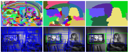
图4 使用SS算法生成候选框的示意图
SS算法基本思想为:
(1)首先通过基于图的图像分割方法(Image Segmentation)将图像分割成很多很多的小块;
(2)使用贪心策略,基于相似度(如颜色相似度、尺寸相似度、纹理相似度等)合并一些区域。
2、RPN算法
SS采用传统特征提取方法,而且非常耗时。是否有更有效方法呢?Faster R-CNN算法中提出一种基于神经网络的生成候选框方法,那就是RPN。
RPN(Region Proposal Networks)层用于生成候选框,并利用softmax判断候选框是前景还是背景,从中选取前景候选框(因为物体一般在前景中),并利用bounding box regression调整候选框的位置,从而得到特征子图,称为proposals。
RPN的工作原理:
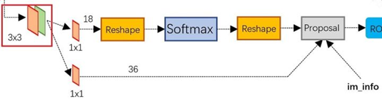
上图展示了RPN网络的具体结构。
首先,经过一次3x3的卷积操作,最后得到了一个channel数目是256的特征图,尺寸和公共特征图相同,我们假设是256 x(H x W)。
然后,经过2条支线:
(1)上面一条支线通过softmax来分类anchors获得前景foreground和背景background(检测目标是foreground),
(2)下面一条支线用于计算anchors的边框偏移量,以获得精确的proposals。
最后的proposal层则负责综合foreground anchors和偏移量获取proposals,同时剔除太小和超出边界的proposals。其实整个网络到了Proposal Layer这里,就完成了相当于目标定位的功能。
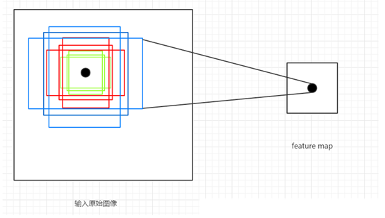
这里涉及一个重要概念anchor:简单地说,RPN依靠一个在共享特征图上滑动的窗口,为每个位置生成9种预先设置好长宽比与面积的目标框(即anchor)。这9种初始anchor包含三种面积(128×128,256×256,512×512),每种面积又包含三种长宽比(1:1,1:2,2:1)。示意图如下图所示:
由于共享特征图的大小约为40×60,所以RPN生成的初始anchor的总数约为20000个(40×60×9)。其实RPN最终就是在原图尺度上,设置了密密麻麻的候选anchor。进而去判断anchor到底是前景还是背景,意思就是判断这个anchor到底有没有覆盖目标,以及为属于前景的anchor进行第一次坐标修正。如何实现坐标修正?具体可参考第三部分的边框回归(Bounding Box Regression)。
3、anchor概述
RPN的目标是代替Selective Search实现候选框的提取,目标检测的实质是对候选框的回归,而网络不可能自动生成任意大小的候选框,因此Anchor的主要意义就在于根据feature map在原图片上划分出很多大小、宽高比不相同的矩形框,RPN会对这些框进行一个粗略的分类(如是否存在目标对象)和回归,选取一些微调过的包含前景的正类别框以及包含背景的负类别框,送入之后的网络结构参与训练。
Anchor的产生过程:
(1)base_size=16 这个参数代表的是网络特征提取过程中图片缩小的倍数,和网络结构有关,ZFNet的缩小倍数为16,表明了最终feature map上一个像素可以映射到原图上16 x 16区域的大小。
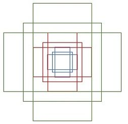
(2)ratios=[0.5,1,2] 这个参数指的是要将16x16的区域,按照1:2,1:1,2:1三种比例进行变换,如下图所示:

(3)scales=2**np.arange(3, 6) 这个参数是要将输入区域的宽和高进行8,16,32三种倍数的放大,如16x16的区域变成(16x8)x(16x8)=128x128的区域,(16x16)x(16x16)=256x256的区域,(16x32)x(16x32)=512x512的区域,如下图所示:
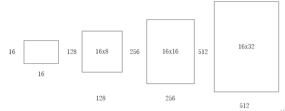
通过以上三个参数,针对于feature map上的任意一个像素点,首先映射到原图片上一个 16 x 16 的区域,然后以这个区域的中心点作为变换中心,将其变为三种宽高比的区域,再分别对这三种区域的面积扩大8,16,32倍,最终一个像素点对应到了原图的9个不同的矩形框,这些框就叫做Anchor,如下图:
注意: 将不完全在图像内部(初始化的anchor的4个坐标点超出图像边界)的anchor都过滤掉,一般过滤后只会有原来1/3左右的anchor。如果不将这部分anchor过滤,则会使训练过程难以收敛。
Anchor是目标检测中的一个重要概念,通常是人为设计的一组框,作为分类(classification)和框回归(bounding box regression)的基准框。
无论是单阶段(single-stage)检测器还是两阶段(two-stage)检测器,都广泛地使用了anchor。例如,
两阶段检测器的第一阶段通常采用 RPN 生成 proposal,是对anchor进行分类和回归的过程,即 anchor -> proposal -> detection bbox;
大部分单阶段检测器是直接对 anchor 进行分类和回归,也就是 anchor -> detection bbox。
常见的生成 anchor 的方式是滑窗(sliding window),也就是首先定义k个特定尺度(scale)和长宽比(aspect ratio)的 anchor,
然后在全图上以一定的步长滑动。这种方式在 Faster R-CNN,YOLO v2+、SSD,RetinaNet 等经典检测方法中被广泛使用。
三、优化候选框
1、交并比(IOU)
通过SS或RPN等方法,最后每类选出的候选框(Region Proposal)比较多,在这些候选框中如何选出质量较好的框?人们想到使用IOU这个度量值。IOU(Intersection Over Union)指标来计算候选框和目标实际标注边界框的重合度。假如我们要计算两个矩形框A和B的IOU,就是它们的交集与并集之比,如下图所示:

矩形框A、B的一个重合度IOU计算公式为:
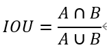
2、非极大值抑制(NMS,Non Maximum Suppression)
通过SS或RPN等方法产生的大量的候选框,这些矩形框有很多是指向同一目标(如下图所示),因此就存在大量冗余的候选。如何减少这些冗余框?NMS就是一个有效方法。
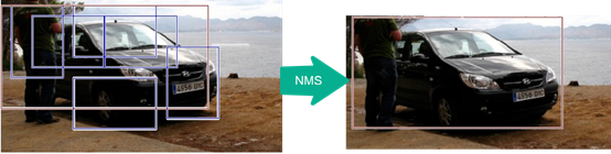
非极大值抑制(Non-Maximum Suppression,以下简称NMS算法)的思想是搜索局部极大值,抑制非极大值元素。就像上图片一样,定位一个车辆,SS或RPN算法对每个目标(如上图中汽车)生成一堆的方框,过滤哪些多余的矩形框,找到那个最佳的矩形框。
非极大值抑制的基本思路为:
先假设有6个候选框,根据分类器类别分类概率做排序,如下图所示:

从小到大分别属于车辆的概率分别为A、B、C、D、E、F。
(1)从最大概率矩形框(即面积最大的框)F开始,分别判断A~E与F的重叠度IOU是否大于某个设定的阈值;
(2)假设B、D与F的重叠度超过阈值,那么就扔掉B、D(因为超过阈值,说明D与F或者B与F,已经有很大部分是重叠的,那我们保留面积最大的F即可,其余小面积的B,D就是多余的,用F完全可以表示一个物体了,所以保留F丢掉B,D);并标记第一个矩形框F,是我们保留下来的。
(3)从剩下的矩形框A、C、E中,选择概率最大的E,然后判断E与A、C的重叠度,重叠度大于一定的阈值,那么就扔掉;并标记E是我们保留下来的第二个矩形框。
(4)一直重复这个过程,找到所有曾经被保留下来的矩形框。
3、边框回归(Bounding Box Regression)
(1)边框回归的主要目的
通过SS或RPN等算法生成的大量候选框,虽然有一部分可以通过NMS等方法过滤一些多余框,但仍然还会存在很多质量不高的框图。如下图所示。
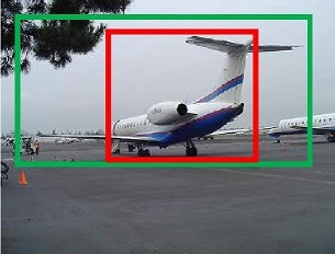
其中红色矩形框(内部这个框)的质量不高(红色的矩形框定位不准(IoU<0.5), 说明这个矩形框没有正确检测出飞机)。需要通过边框回归进行修改。此外,训练时作为有监督学习,也需要通过边框回归使预测框,通过迭代不断向目标框(Ground Truth)靠近。
(2)边框回归的主要原理
下图所示,红色的框A代表生成的候选框(即positive Anchors),绿色的框G代表目标框(Ground Truth),接下来需要基于A和G,找到一种映射关系得到一个预测框G’通过迭代使G’不断接近目标框G。这个过程用数学符合可表示为:,


(3)如何找到这个对应关系F?
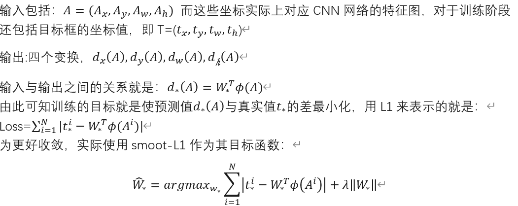
如何通过变换F实现从上图中的矩形框A变为矩形框G’呢? 比较简单的思路就是: 平移+放缩,具体实现步骤如下:

以认为d_\astA(这里*表示x,y,w,h)变换是一种线性变换, 如此就可以用线性回归来建模对矩形框进行微调。线性回归就是给定输入的特征向量X, 学习一组参数W, 使得经过线性回归后的值跟真实值 G(Ground Truth)非常接近. 即G≈WX 。 那么 anchor Bounding-box 中的输入以及输出分别是什么呢?
(4)边框回归为何只能微调?
要使用线性回归,要求anchor A与G相乘较小,否则这些变换将可能变成复杂的非线性变换。
(5)边框回归主要应用
在RPN生成Proposal的过程中,最后输出时也使用边框回归使预测框不断向目标框逼近。
(6)改进空间
YOLO v2提出一种直接预测位置坐标的方法。之前的坐标回归实际上回归的不是坐标点,而是需要对预测结果做一个变换才能得到坐标点,这种方法在充分利用目的对象的位置信息方面效率打了较大折扣,为更好利用目标对象的位置信息,YOLO v2采用目标对象的中心坐标及左上角的方法,具体可参考下图:
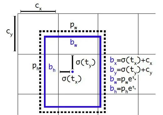
其中p_w,P_h为anchor box的宽和高,t_x,\ t_y,t_w,t_h为预测边界框的坐标值,σ是sigmoid函数。C_x,C_y为是当前网格左上角到图像左上角的距离,需要将网格大小归一化,即令一个网格的宽=1,高=1。
四、模型优化
1、SPP Net
SPP-Net 是何恺明、孙健等人的作品。SPP-Net 的主要创新点就是SPP,即Spatial pyramid pooling,空间金字塔池化。该方案解决了R-CNN 中每个region proposal 都要过一次CNN 的缺点,从而提升了效率,并且避免了为了适应CNN 的输入尺寸而图像缩放导致的目标形状失真的问题。我们通常看到的RoI pooling是SPP-net的一种变换版本。
2、FPN
FPN 全称Feature Pyramid Network,其主要思路是通过特征层面(即feature map)的转换,生成语义和低层信息都很丰富的特征金字塔,用于预测
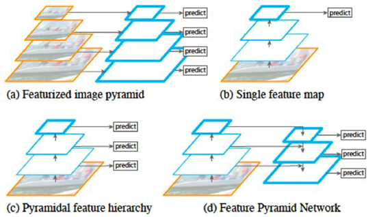
如图所示,(a) 表示的是图像金字塔(image pyramid),即对图像进行放缩,不同的尺度分别进行预测。这种方法在目标检测里较为常用,但是速度较慢,因为每次需要对不同尺度的图像分别过一次CNN 进行训练。(b)表示的是单一feature map 的预测。由于图像金字塔速度太慢,索性直接只采用最后一层输出进行预测,但这样做同时也丢失了很多信息。(c) 表示的是各个scale 的feature map 分别进行预测,但是各个层次之间(不同scale)没有交互。SSD 模型中就是采用了这种策略,将不同尺度的bbox 分配到代表不同scale 的feature map上。(d) 即为这里要将的FPN 网络,即特征金字塔。这种方式通过将所有scale 的feature map 进行打通和结合,兼顾了速度和准确率。
如何进行横向连接和融合?如下。把高层特征做2倍上采样,然后将其和对应的前一层特征结合,注意前一层特征经过 1*1 的卷积改变维度使得可以用加法进行融合。值得一提的是,这只是其中一种融合方式,当然也可以做通道上的 concat
FPN 在每两层之间为一个buiding block,结构如下:

FPN 的block 结构分为两个部分,一个自顶向下通路(top-down pathway),另一个是侧边通路(lateral pathway)。所谓自顶向下通路,具体指的是上一个小尺寸的feature map(语义更高层)做2 倍上采样,并连接到下一层。而侧边通路则指的是下面的feature map(高分辨率低语义)先利用一个1×1 的卷积核进行通道压缩,然后和上面下来的采样后结果进行合并。合并方式为逐元素相加(element-wise addition)。合并之后的结果在通过一个3×3 的卷积核进行处理,得到该scale 下的feature map。
FPN 并不是一个目标检测框架,它的这种结构可以融入到其他的目标检测框架中,去提升检测器的性能。截至现在,FPN 已经可以说成为目标检测框架中必备的结构了。
使用Transformer来提升模型的性能
最近几年,Transformer体系结构已成为自然语言处理任务的实际标准,
但其在计算机视觉中的应用还受到限制。在视觉上,注意力要么与卷积网络结合使用,
要么用于替换卷积网络的某些组件,同时将其整体结构保持在适当的位置。2020年10月22日,谷歌人工智能研究院发表一篇题为“An Image is Worth 16x16 Words: Transformers for Image Recognition at Scale”的文章。文章将图像切割成一个个图像块,组成序列化的数据输入Transformer执行图像分类任务。当对大量数据进行预训练并将其传输到多个中型或小型图像识别数据集(如ImageNet、CIFAR-100、VTAB等)时,与目前的卷积网络相比,Vision Transformer(ViT)获得了出色的结果,同时所需的计算资源也大大减少。
这里我们以ViT我模型,实现对数据CiFar10的分类工作,模型性能得到进一步的提升。
1、导入模型
|
1 2 3 4 5 6 7 8 9 10 |
import os import math import numpy as np import pickle as p import tensorflow as tf from tensorflow import keras import matplotlib.pyplot as plt from tensorflow.keras import layers import tensorflow_addons as tfa %matplotlib inline |
这里使用了TensorFlow_addons模块,它实现了核心 TensorFlow 中未提供的新功能。
tensorflow_addons的安装要注意与tf的版本对应关系,请参考:
https://github.com/tensorflow/addons。
安装addons时要注意其版本与tensorflow版本的对应,具体关系以上这个链接有。
2、定义加载函数
|
1 2 3 4 5 6 7 8 9 10 11 12 13 14 15 16 17 18 19 20 21 |
def load_CIFAR_data(data_dir): """load CIFAR data""" images_train=[] labels_train=[] for i in range(5): f=os.path.join(data_dir,'data_batch_%d' % (i+1)) print('loading ',f) # 调用 load_CIFAR_batch( )获得批量的图像及其对应的标签 image_batch,label_batch=load_CIFAR_batch(f) images_train.append(image_batch) labels_train.append(label_batch) Xtrain=np.concatenate(images_train) Ytrain=np.concatenate(labels_train) del image_batch ,label_batch Xtest,Ytest=load_CIFAR_batch(os.path.join(data_dir,'test_batch')) print('finished loadding CIFAR-10 data') # 返回训练集的图像和标签,测试集的图像和标签 return (Xtrain,Ytrain),(Xtest,Ytest) |
3、定义批量加载函数
|
1 2 3 4 5 6 7 8 9 10 11 12 13 14 15 16 17 18 19 20 |
def load_CIFAR_batch(filename): """ load single batch of cifar """ with open(filename, 'rb')as f: # 一个样本由标签和图像数据组成 # (3072=32x32x3) # ... # data_dict = p.load(f, encoding='bytes') images= data_dict[b'data'] labels = data_dict[b'labels'] # 把原始数据结构调整为: BCWH images = images.reshape(10000, 3, 32, 32) # tensorflow处理图像数据的结构:BWHC # 把通道数据C移动到最后一个维度 images = images.transpose (0,2,3,1) labels = np.array(labels) return images, labels |
4、加载数据
|
1 2 |
data_dir = r'C:\Users\wumg\jupyter-ipynb\data\cifar-10-batches-py' (x_train,y_train),(x_test,y_test) = load_CIFAR_data(data_dir) |
把数据转换为dataset格式
|
1 2 |
train_dataset = tf.data.Dataset.from_tensor_slices((x_train, y_train)) test_dataset = tf.data.Dataset.from_tensor_slices((x_test, y_test)) |
5、定义数据预处理及训练模型的一些超参数
|
1 2 3 4 5 6 7 8 9 10 11 12 13 14 15 16 17 18 19 |
num_classes = 10 input_shape = (32, 32, 3) learning_rate = 0.001 weight_decay = 0.0001 batch_size = 256 num_epochs = 10 image_size = 72 # We'll resize input images to this size patch_size = 6 # Size of the patches to be extract from the input images num_patches = (image_size // patch_size) ** 2 projection_dim = 64 num_heads = 4 transformer_units = [ projection_dim * 2, projection_dim, ] # Size of the transformer layers transformer_layers = 8 mlp_head_units = [2048, 1024] # Size of the dense layers of the final classifier |
6、定义数据增强模型
|
1 2 3 4 5 6 7 8 9 10 11 12 13 14 15 |
data_augmentation = keras.Sequential( [ layers.experimental.preprocessing.Normalization(), layers.experimental.preprocessing.Resizing(image_size, image_size), layers.experimental.preprocessing.RandomFlip("horizontal"), layers.experimental.preprocessing.RandomRotation(factor=0.02), layers.experimental.preprocessing.RandomZoom( height_factor=0.2, width_factor=0.2 ), ], name="data_augmentation", ) # 使预处理层的状态与正在传递的数据相匹配 #Compute the mean and the variance of the training data for normalization. data_augmentation.layers[0].adapt(x_train) |
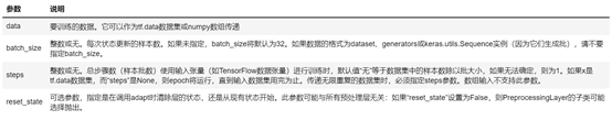
预处理层是在模型训练开始之前计算其状态的层。他们在训练期间不会得到更新。大多数预处理层为状态计算实现了adapt()方法。
adapt(data, batch_size=None, steps=None, reset_state=True)该函数参数说明如下:
7、构建模型
7.1 构建多层感知器(MLP)
|
1 2 3 4 5 |
def mlp(x, hidden_units, dropout_rate): for units in hidden_units: x = layers.Dense(units, activation=tf.nn.gelu)(x) x = layers.Dropout(dropout_rate)(x) return x |
7.2 创建一个类似卷积层的patch层
|
1 2 3 4 5 6 7 8 9 10 11 12 13 14 15 16 17 |
class Patches(layers.Layer): def __init__(self, patch_size): super(Patches, self).__init__() self.patch_size = patch_size def call(self, images): batch_size = tf.shape(images)[0] patches = tf.image.extract_patches( images=images, sizes=[1, self.patch_size, self.patch_size, 1], strides=[1, self.patch_size, self.patch_size, 1], rates=[1, 1, 1, 1], padding="VALID", ) patch_dims = patches.shape[-1] patches = tf.reshape(patches, [batch_size, -1, patch_dims]) return patches |
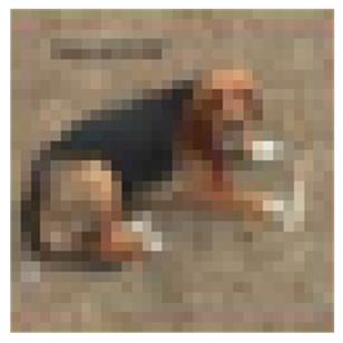
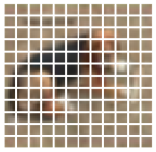
7.3 查看由patch层随机生成的图像块
|
1 2 3 4 5 6 7 8 9 10 11 12 13 14 15 16 17 18 19 20 21 22 23 |
import matplotlib.pyplot as plt plt.figure(figsize=(4, 4)) image = x_train[np.random.choice(range(x_train.shape[0]))] plt.imshow(image.astype("uint8")) plt.axis("off") resized_image = tf.image.resize( tf.convert_to_tensor([image]), size=(image_size, image_size) ) patches = Patches(patch_size)(resized_image) print(f"Image size: {image_size} X {image_size}") print(f"Patch size: {patch_size} X {patch_size}") print(f"Patches per image: {patches.shape[1]}") print(f"Elements per patch: {patches.shape[-1]}") n = int(np.sqrt(patches.shape[1])) plt.figure(figsize=(4, 4)) for i, patch in enumerate(patches[0]): ax = plt.subplot(n, n, i + 1) patch_img = tf.reshape(patch, (patch_size, patch_size, 3)) plt.imshow(patch_img.numpy().astype("uint8")) plt.axis("off") |
运行结果
Image size: 72 X 72
Patch size: 6 X 6
Patches per image: 144
Elements per patch: 108
7.4构建patch 编码层( encoding layer)
|
1 2 3 4 5 6 7 8 9 10 11 12 13 14 15 16 |
class PatchEncoder(layers.Layer): def __init__(self, num_patches, projection_dim): super(PatchEncoder, self).__init__() self.num_patches = num_patches #一个全连接层,其输出维度为projection_dim,没有指明激活函数 self.projection = layers.Dense(units=projection_dim) #定义一个嵌入层,这是一个可学习的层 #输入维度为num_patches,输出维度为projection_dim self.position_embedding = layers.Embedding( input_dim=num_patches, output_dim=projection_dim ) def call(self, patch): positions = tf.range(start=0, limit=self.num_patches, delta=1) encoded = self.projection(patch) + self.position_embedding(positions) return encoded |
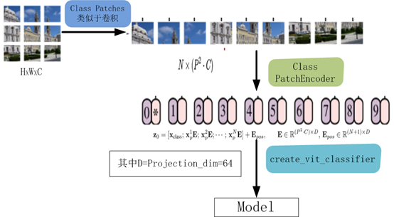
7.5构建ViT模型
|
1 2 3 4 5 6 7 8 9 10 11 12 13 14 15 16 17 18 19 20 21 22 23 24 25 26 27 28 29 30 31 32 33 34 35 36 37 38 |
def create_vit_classifier(): inputs = layers.Input(shape=input_shape) # Augment data. augmented = data_augmentation(inputs) #augmented = augmented_train_batches(inputs) # Create patches. patches = Patches(patch_size)(augmented) # Encode patches. encoded_patches = PatchEncoder(num_patches, projection_dim)(patches) # Create multiple layers of the Transformer block. for _ in range(transformer_layers): # Layer normalization 1. x1 = layers.LayerNormalization(epsilon=1e-6)(encoded_patches) # Create a multi-head attention layer. attention_output = layers.MultiHeadAttention( num_heads=num_heads, key_dim=projection_dim, dropout=0.1 )(x1, x1) # Skip connection 1. x2 = layers.Add()([attention_output, encoded_patches]) # Layer normalization 2. x3 = layers.LayerNormalization(epsilon=1e-6)(x2) # MLP. x3 = mlp(x3, hidden_units=transformer_units, dropout_rate=0.1) # Skip connection 2. encoded_patches = layers.Add()([x3, x2]) # Create a [batch_size, projection_dim] tensor. representation = layers.LayerNormalization(epsilon=1e-6)(encoded_patches) representation = layers.Flatten()(representation) representation = layers.Dropout(0.5)(representation) # Add MLP. features = mlp(representation, hidden_units=mlp_head_units, dropout_rate=0.5) # Classify outputs. logits = layers.Dense(num_classes)(features) # Create the Keras model. model = keras.Model(inputs=inputs, outputs=logits) return model |
该模型的处理流程如下图所示
8、编译、训练模型
|
1 2 3 4 5 6 7 8 9 10 11 12 13 14 15 16 17 18 19 20 21 22 23 24 25 26 27 28 29 30 31 32 33 34 35 36 37 38 |
def run_experiment(model): optimizer = tfa.optimizers.AdamW( learning_rate=learning_rate, weight_decay=weight_decay ) model.compile( optimizer=optimizer, loss=keras.losses.SparseCategoricalCrossentropy(from_logits=True), metrics=[ keras.metrics.SparseCategoricalAccuracy(name="accuracy"), keras.metrics.SparseTopKCategoricalAccuracy(5, name="top-5-accuracy"), ], ) #checkpoint_filepath = r".\tmp\checkpoint" checkpoint_filepath ="model_bak.hdf5" checkpoint_callback = keras.callbacks.ModelCheckpoint( checkpoint_filepath, monitor="val_accuracy", save_best_only=True, save_weights_only=True, ) history = model.fit( x=x_train, y=y_train, batch_size=batch_size, epochs=num_epochs, validation_split=0.1, callbacks=[checkpoint_callback], ) model.load_weights(checkpoint_filepath) _, accuracy, top_5_accuracy = model.evaluate(x_test, y_test) print(f"Test accuracy: {round(accuracy * 100, 2)}%") print(f"Test top 5 accuracy: {round(top_5_accuracy * 100, 2)}%") return history |
实例化类,运行模型
|
1 2 |
vit_classifier = create_vit_classifier() history = run_experiment(vit_classifier) |
运行结果
Epoch 1/10
176/176 [==============================] - 68s 333ms/step - loss: 2.6394 - accuracy: 0.2501 - top-5-accuracy: 0.7377 - val_loss: 1.5331 - val_accuracy: 0.4580 - val_top-5-accuracy: 0.9092
Epoch 2/10
176/176 [==============================] - 58s 327ms/step - loss: 1.6359 - accuracy: 0.4150 - top-5-accuracy: 0.8821 - val_loss: 1.2714 - val_accuracy: 0.5348 - val_top-5-accuracy: 0.9464
Epoch 3/10
176/176 [==============================] - 58s 328ms/step - loss: 1.4332 - accuracy: 0.4839 - top-5-accuracy: 0.9210 - val_loss: 1.1633 - val_accuracy: 0.5806 - val_top-5-accuracy: 0.9616
Epoch 4/10
176/176 [==============================] - 58s 329ms/step - loss: 1.3253 - accuracy: 0.5280 - top-5-accuracy: 0.9349 - val_loss: 1.1010 - val_accuracy: 0.6112 - val_top-5-accuracy: 0.9572
Epoch 5/10
176/176 [==============================] - 58s 330ms/step - loss: 1.2380 - accuracy: 0.5626 - top-5-accuracy: 0.9411 - val_loss: 1.0212 - val_accuracy: 0.6400 - val_top-5-accuracy: 0.9690
Epoch 6/10
176/176 [==============================] - 58s 330ms/step - loss: 1.1486 - accuracy: 0.5945 - top-5-accuracy: 0.9520 - val_loss: 0.9698 - val_accuracy: 0.6602 - val_top-5-accuracy: 0.9718
Epoch 7/10
176/176 [==============================] - 58s 330ms/step - loss: 1.1208 - accuracy: 0.6060 - top-5-accuracy: 0.9558 - val_loss: 0.9215 - val_accuracy: 0.6724 - val_top-5-accuracy: 0.9790
Epoch 8/10
176/176 [==============================] - 58s 330ms/step - loss: 1.0643 - accuracy: 0.6248 - top-5-accuracy: 0.9621 - val_loss: 0.8709 - val_accuracy: 0.6944 - val_top-5-accuracy: 0.9768
Epoch 9/10
176/176 [==============================] - 58s 330ms/step - loss: 1.0119 - accuracy: 0.6446 - top-5-accuracy: 0.9640 - val_loss: 0.8290 - val_accuracy: 0.7142 - val_top-5-accuracy: 0.9784
Epoch 10/10
176/176 [==============================] - 58s 330ms/step - loss: 0.9740 - accuracy: 0.6615 - top-5-accuracy: 0.9666 - val_loss: 0.8175 - val_accuracy: 0.7096 - val_top-5-accuracy: 0.9806
313/313 [==============================] - 9s 27ms/step - loss: 0.8514 - accuracy: 0.7032 - top-5-accuracy: 0.9773
Test accuracy: 70.32%
Test top 5 accuracy: 97.73%
In [15]:
从结果看可以来看,测试精度已达70%,这是一个较大提升!
9、查看运行结果
|
1 2 3 4 5 6 7 8 9 10 11 12 13 14 15 16 17 18 19 20 21 22 23 24 |
acc = history.history['accuracy'] val_acc = history.history['val_accuracy'] loss = history.history['loss'] val_loss =history.history['val_loss'] plt.figure(figsize=(8, 8)) plt.subplot(2, 1, 1) plt.plot(acc, label='Training Accuracy') plt.plot(val_acc, label='Validation Accuracy') plt.legend(loc='lower right') plt.ylabel('Accuracy') plt.ylim([min(plt.ylim()),1.1]) plt.title('Training and Validation Accuracy') plt.subplot(2, 1, 2) plt.plot(loss, label='Training Loss') plt.plot(val_loss, label='Validation Loss') plt.legend(loc='upper right') plt.ylabel('Cross Entropy') plt.ylim([-0.1,4.0]) plt.title('Training and Validation Loss') plt.xlabel('epoch') plt.show() |
运行结果
使用数据增强来提升模型的性能
1、导入模型
|
1 2 3 4 5 6 7 8 |
import os import math import numpy as np import pickle as p import tensorflow as tf from tensorflow import keras import matplotlib.pyplot as plt %matplotlib inline |
2、定义加载函数
|
1 2 3 4 5 6 7 8 9 10 11 12 13 14 15 16 17 18 19 20 21 |
def load_CIFAR_data(data_dir): """load CIFAR data""" images_train=[] labels_train=[] for i in range(5): f=os.path.join(data_dir,'data_batch_%d' % (i+1)) print('loading ',f) # 调用 load_CIFAR_batch( )获得批量的图像及其对应的标签 image_batch,label_batch=load_CIFAR_batch(f) images_train.append(image_batch) labels_train.append(label_batch) Xtrain=np.concatenate(images_train) Ytrain=np.concatenate(labels_train) del image_batch ,label_batch Xtest,Ytest=load_CIFAR_batch(os.path.join(data_dir,'test_batch')) print('finished loadding CIFAR-10 data') # 返回训练集的图像和标签,测试集的图像和标签 return (Xtrain,Ytrain),(Xtest,Ytest) |
3、定义批量加载函数
|
1 2 3 4 5 6 7 8 9 10 11 12 13 14 15 16 17 18 19 20 |
def load_CIFAR_batch(filename): """ load single batch of cifar """ with open(filename, 'rb')as f: # 一个样本由标签和图像数据组成 # (3072=32x32x3) # ... # data_dict = p.load(f, encoding='bytes') images= data_dict[b'data'] labels = data_dict[b'labels'] # 把原始数据结构调整为: BCWH images = images.reshape(10000, 3, 32, 32) # tensorflow处理图像数据的结构:BWHC # 把通道数据C移动到最后一个维度 images = images.transpose (0,2,3,1) labels = np.array(labels) return images, labels |
4、加载数据
|
1 2 |
data_dir = r'C:\Users\wumg\jupyter-ipynb\data\cifar-10-batches-py' (x_train,y_train),(x_test,y_test) = load_CIFAR_data(data_dir) |
把数据转换为dataset格式
|
1 2 |
train_dataset = tf.data.Dataset.from_tensor_slices((x_train, y_train)) test_dataset = tf.data.Dataset.from_tensor_slices((x_test, y_test)) |
5、定义数据增强方法
|
1 2 3 4 5 6 7 8 9 10 11 12 13 14 15 16 17 18 19 20 21 22 23 24 25 26 27 28 29 30 31 32 33 34 |
def convert(image, label): image = tf.image.convert_image_dtype(image, tf.float32) return image, label def augment(image, label): image, label = convert(image, label) #image = tf.image.convert_image_dtype(image, tf.float32) image = tf.image.resize_with_crop_or_pad(image, 34,34) # 四周各加3像素 image = tf.image.random_crop(image, size=[32,32,3]) # 随机裁剪成28*28大小 image = tf.image.random_brightness(image, max_delta=0.5) # 随机增加亮度 return image, label batch_size = 64 augmented_train_batches = (train_dataset #.take(num_examples) .cache() # .repeat() .shuffle(5000) .map(augment, num_parallel_calls=tf.data.experimental.AUTOTUNE) .batch(batch_size) .prefetch(tf.data.experimental.AUTOTUNE)) non_augmented_train_batches = (train_dataset .cache() # .repeat() .shuffle(5000) .map(convert, num_parallel_calls=tf.data.experimental.AUTOTUNE) .batch(batch_size) .prefetch(tf.data.experimental.AUTOTUNE)) validation_batches = (test_dataset .map(convert, num_parallel_calls=tf.data.experimental.AUTOTUNE) .batch(2*batch_size)) |
6、构建模型
|
1 2 3 4 5 6 7 8 9 10 11 12 13 14 15 16 17 18 19 20 21 22 23 24 25 26 27 28 29 30 31 32 33 34 |
class MyCNN(tf.keras.Model): def __init__(self): super().__init__() self.conv1 = tf.keras.layers.Conv2D( filters=32, # 卷积层神经元(卷积核)数目 kernel_size=[3, 3], # 感受野大小 padding='same', # padding策略(vaild 或 same) activation=tf.nn.relu # 激活函数 ) self.pool1 = tf.keras.layers.MaxPool2D(pool_size=[2, 2], strides=2) self.conv2 = tf.keras.layers.Conv2D( filters=64, kernel_size=[3, 3], padding='same', activation=tf.nn.relu ) self.pool2 = tf.keras.layers.MaxPool2D(pool_size=[2, 2], strides=2) self.flatten = tf.keras.layers.Reshape(target_shape=(8 * 8 * 64,)) self.dense1 = tf.keras.layers.Dense(units=256, activation=tf.nn.relu) self.dense2 = tf.keras.layers.Dense(units=10) def call(self, inputs): x = self.conv1(inputs) # [batch_size, 32, 32, 3] x = self.pool1(x) # [batch_size, 32, 32, 32] x = self.conv2(x) # [batch_size, 16, 16, 64] x = self.pool2(x) # [batch_size, 8, 8, 64] x = self.flatten(x) # [batch_size, 8 * 8 * 64] x = self.dense1(x) # [batch_size, 256] x = self.dense2(x) # [batch_size, 10] output = tf.nn.softmax(x) return output def model01(self): x = tf.keras.Input(shape=(32, 32, 3)) return tf.keras.Model(inputs=[x], outputs=self.call(x)) |
生成实例
|
1 |
model_no_augment = MyCNN() |
查看模型详细结构
|
1 |
model_no_augment.model01().summary() |
7、编译模型
|
1 |
model_no_augment.compile(optimizer='adam',loss='sparse_categorical_crossentropy',metrics=['accuracy']) |
8、训练模型
为便于比较,这里先不使用数据增强方法
|
1 2 |
epochs = 10 history_non_augment = model_no_augment.fit(non_augmented_train_batches,epochs=epochs,validation_data=validation_batches) |
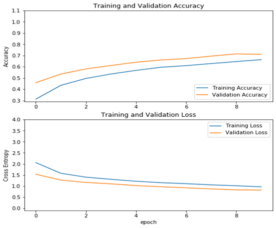
9、查看运行结果
|
1 2 3 4 5 6 7 8 9 10 11 12 13 14 15 16 17 18 19 20 21 22 23 24 |
acc = history_non_augment.history['accuracy'] val_acc = history_non_augment.history['val_accuracy'] loss = history_non_augment.history['loss'] val_loss = history_non_augment.history['val_loss'] plt.figure(figsize=(8, 8)) plt.subplot(2, 1, 1) plt.plot(acc, label='Training Accuracy') plt.plot(val_acc, label='Validation Accuracy') plt.legend(loc='lower right') plt.ylabel('Accuracy') plt.ylim([min(plt.ylim()),1.1]) plt.title('Training and Validation Accuracy') plt.subplot(2, 1, 2) plt.plot(loss, label='Training Loss') plt.plot(val_loss, label='Validation Loss') plt.legend(loc='upper right') plt.ylabel('Cross Entropy') plt.ylim([-0.1,1.0]) plt.title('Training and Validation Loss') plt.xlabel('epoch') plt.show() |
运行结果

10、使用数据增强方法
|
1 2 3 4 5 |
model_augment = MyCNN() model_augment.compile(optimizer='adam',loss='sparse_categorical_crossentropy',metrics=['accuracy']) history_with_augment = model_augment.fit(augmented_train_batches,epochs=epochs,validation_data=validation_batches) |
11、查看使用数据增强的运行结果
|
1 2 3 4 5 6 7 8 9 10 11 12 13 14 15 16 17 18 19 20 21 22 23 24 |
acc = history_with_augment.history['accuracy'] val_acc = history_with_augment.history['val_accuracy'] loss = history_with_augment.history['loss'] val_loss = history_with_augment.history['val_loss'] plt.figure(figsize=(8, 8)) plt.subplot(2, 1, 1) plt.plot(acc, label='Training Accuracy') plt.plot(val_acc, label='Validation Accuracy') plt.legend(loc='lower right') plt.ylabel('Accuracy') plt.ylim([min(plt.ylim()),1.1]) plt.title('Training and Validation Accuracy') plt.subplot(2, 1, 2) plt.plot(loss, label='Training Loss') plt.plot(val_loss, label='Validation Loss') plt.legend(loc='upper right') plt.ylabel('Cross Entropy') plt.ylim([-0.1,1.0]) plt.title('Training and Validation Loss') plt.xlabel('epoch') plt.show() |
运行结果
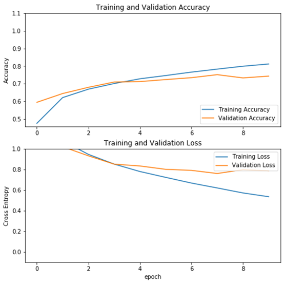
12、结果分析
从不使用数据增强与使用数据增强方法的结果可以看出,使用数据增强方法后,模型性能有提升(未使用数据增强的验证精度为71%,使用数据增强方法后,验证精度提升到74%),而且模型的泛化能力也有提高(使用数据增强方法后,训练与验证精度曲线靠得较近)。